
Batteries
More nickel, more energy, shorter life: layered NMC cathodes
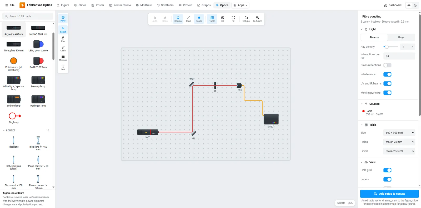
NMC111, NMC622 and NMC811 side by side: synthesis scheme, voltage profiles, capacity retention and why Ni-rich particles crack.
Open in Research PosterLabCanvas puts figures, slides, posters, 3D scenes, protein views and graphs in one workspace that runs in your browser. Every object is drawn by a generator you can adjust.
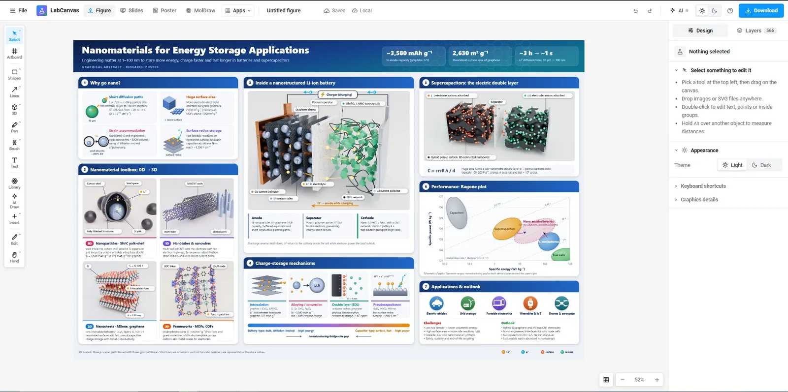
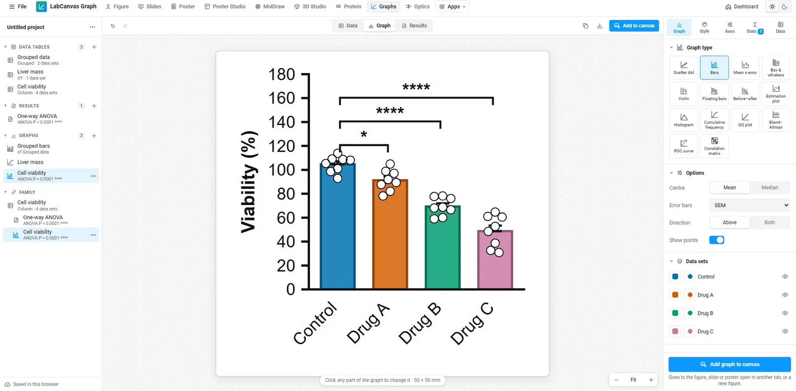
70 graph types, from scatter dot plots, bars with SD/SEM error bars, box and violin plots to grouped bars, Kaplan–Meier curves, volcano plots and heat maps. Run t tests (paired, unpaired, Welch), one- and two-way ANOVA with Tukey, Dunnett, Šídák or Bonferroni post hoc tests, Mann–Whitney, Wilcoxon and Kruskal–Wallis, nonlinear curve fitting (dose–response IC50/EC50, Michaelis–Menten, exponential, Gaussian), linear regression, Pearson and Spearman correlation, log-rank and Cox survival, chi-square and Fisher tests. Significance stars drawn for you, Prism files open (.prism and .pzfx), TIFF export for journals.
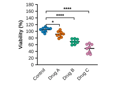 Scatter dot plot
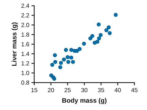 XY scatter
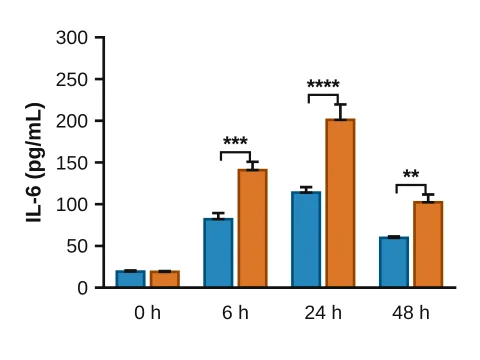 Grouped bars
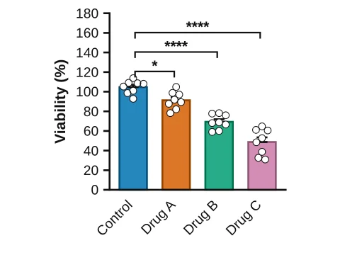 Bars with points
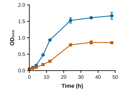 Line graph
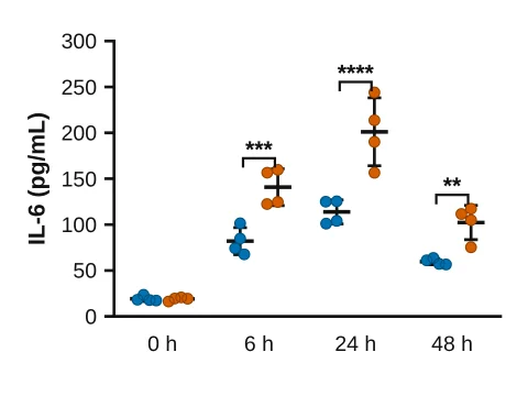 Grouped scatter
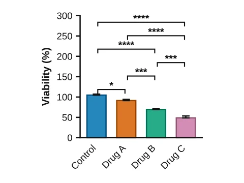 Bar chart
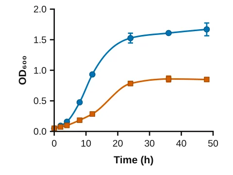 Smooth curve
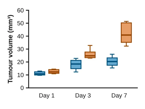 Grouped box plot
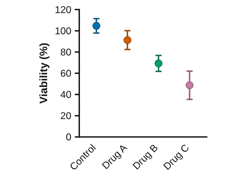 Mean ± SD
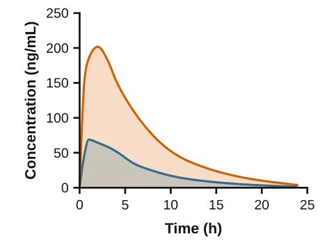 Area chart
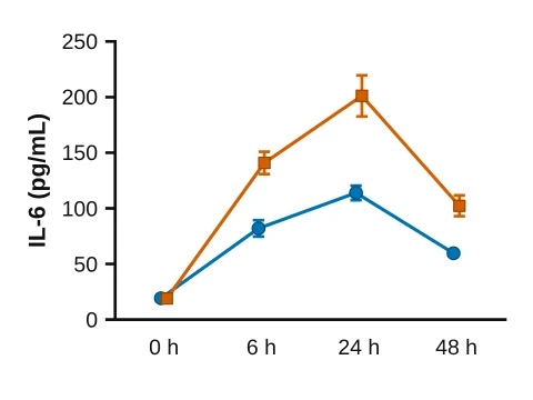 Time course
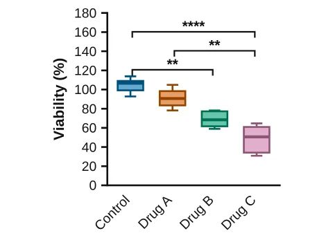 Box & whiskers
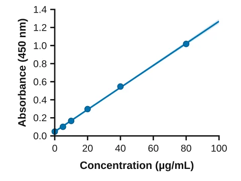 Linear regression
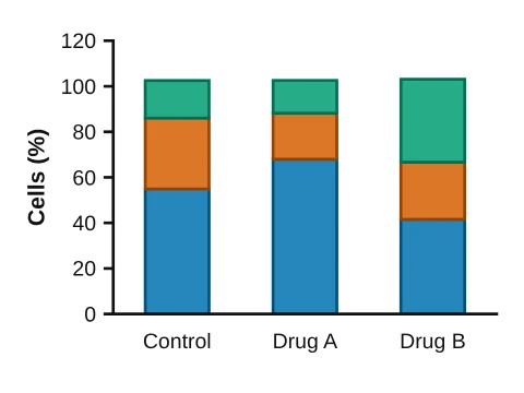 Stacked bars
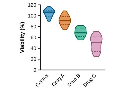 Violin plot
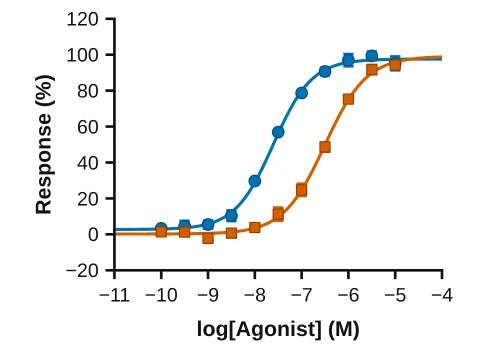 Dose–response curve
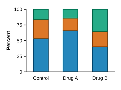 100% stacked bars
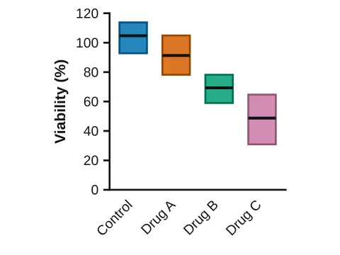 Floating bars
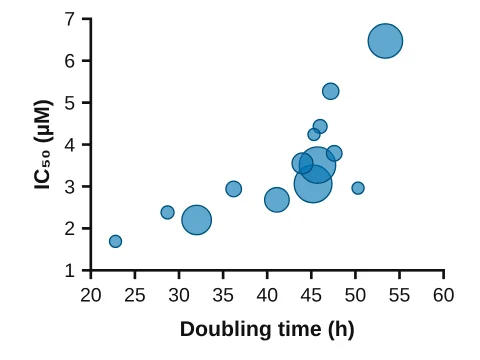 Bubble plot
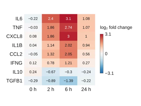 Heat map
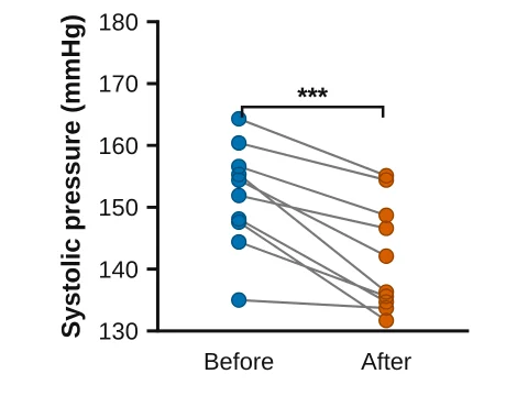 Before–after
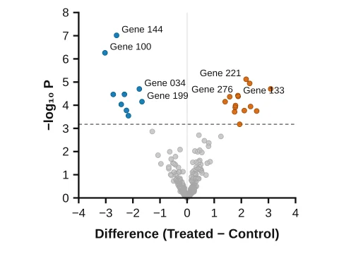 Volcano plot
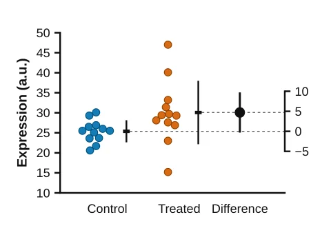 Estimation plot
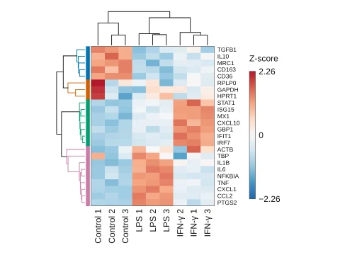 Clustered heat map
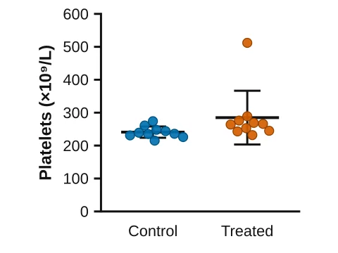 Find outliers
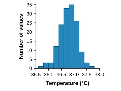 Histogram
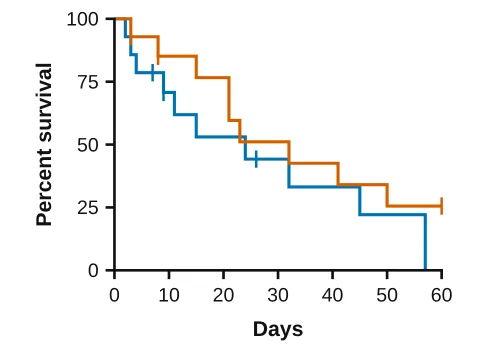 Kaplan–Meier
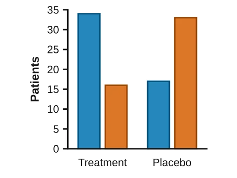 Counts by group
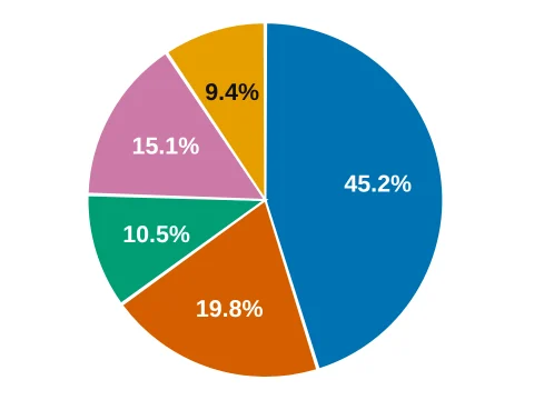 Pie chart
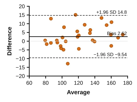 Bland–Altman
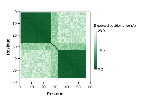 Predicted aligned error (PAE)
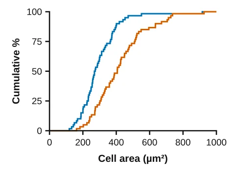 Cumulative frequency
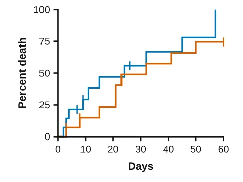 Cumulative incidence
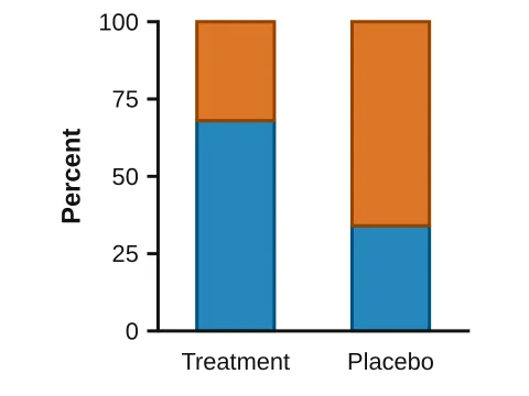 Stacked percentages
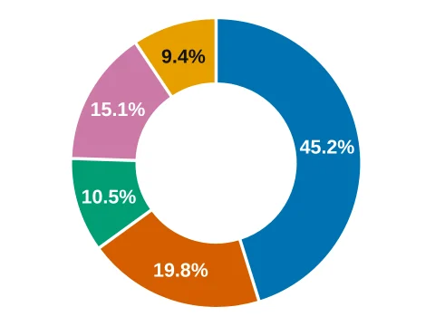 Donut chart
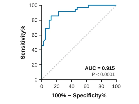 ROC curve
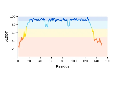 Per-residue confidence (pLDDT)
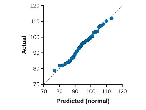 QQ plot
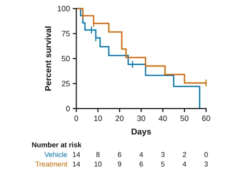 Kaplan–Meier with numbers at risk
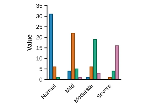 Rater agreement (kappa)
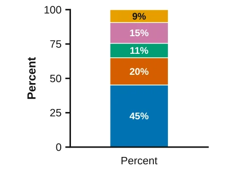 100% bar
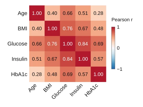 Correlation matrix
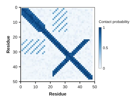 Contact map
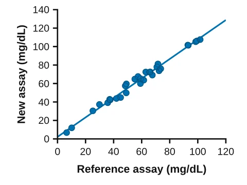 Method comparison (Deming)
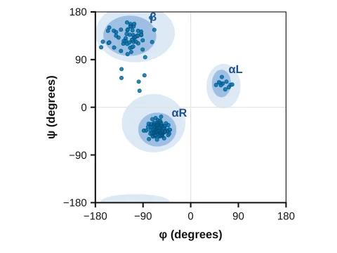 Ramachandran plot
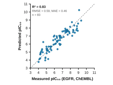 Parity plot (ML model)
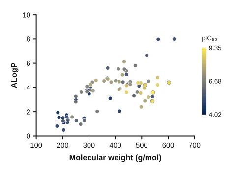 Chemical space map
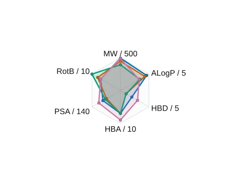 Property radar (drug-likeness)
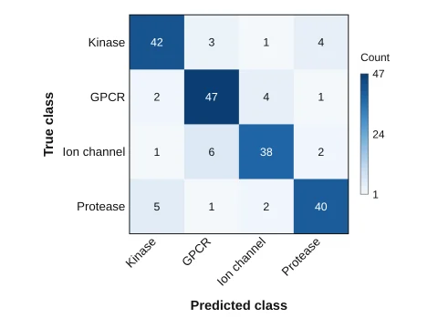 Confusion matrix
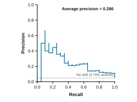 Precision–recall curve
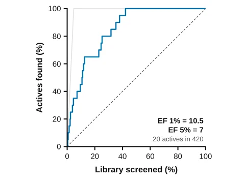 Enrichment curve
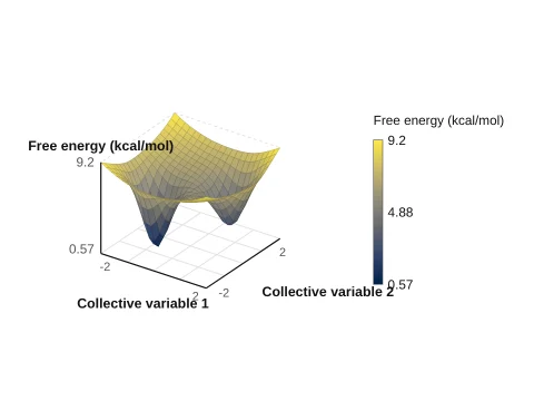 3D free energy landscape
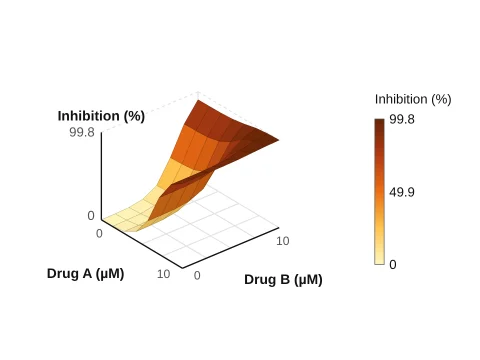 Drug combination surface
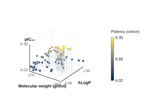 3D scatter
Polymers and gels, membranes and porous solids, nanoparticles, cells and viruses, frameworks, batteries, devices, instruments and AI-driven labs, drawn by generators: change a setting and the drawing follows.
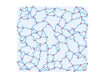
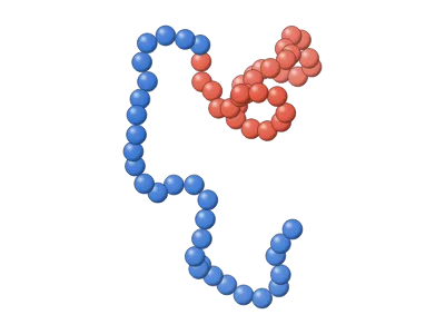 Polymer chain architectures (3D)
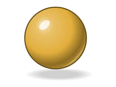 Nanoparticle (3D)
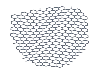
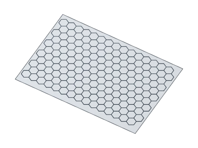 Graphene sheet
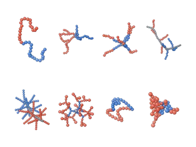 Polymer architectures: linear to hyperbranched (3D)
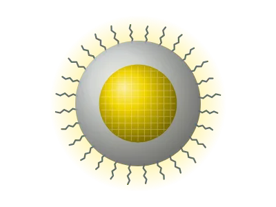
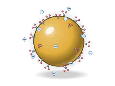 Gold NP, citrate-capped
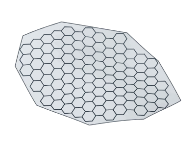 Graphene flake
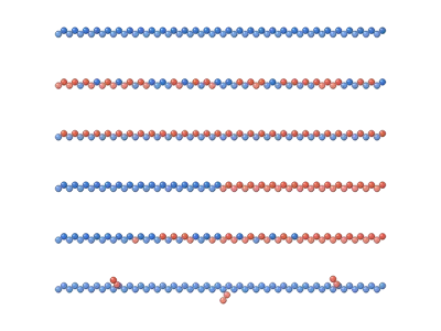 Copolymer sequences: random, alternating, block, gradient, graft
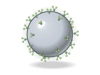 Silver NP, phytochemical capping
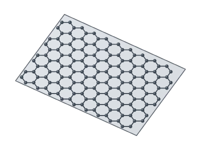 Graphene (ball and stick)
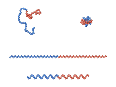 Chain conformations: coil, globule, extended, helix (3D)
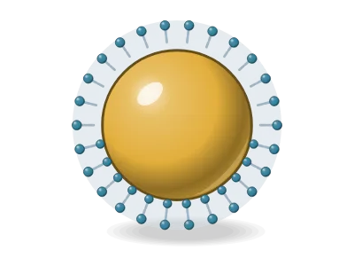 CTAB-capped gold seed
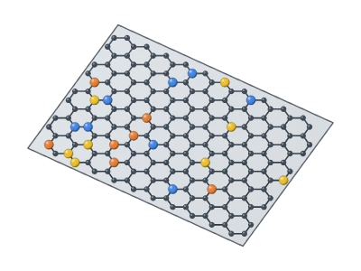 Doped graphene (N, S, Fe)
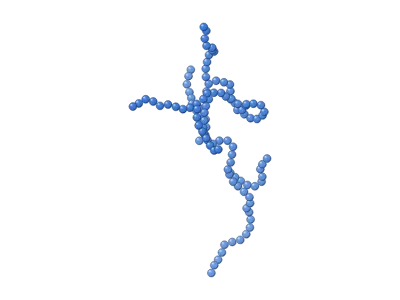 Branched polymer with long-chain branches (3D)
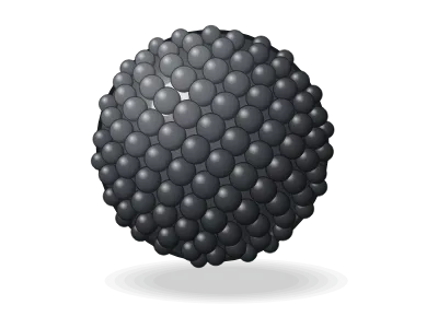 Magnetite NP (Fe₃O₄)
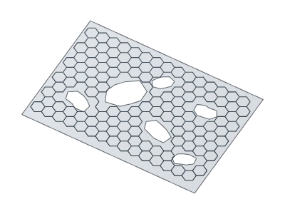 Porous graphene
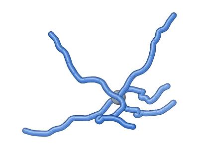 Star polymer (3D)
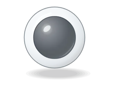 Fe₃O₄@SiO₂ core–shell
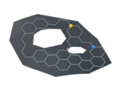 Doped carbon nanosheet
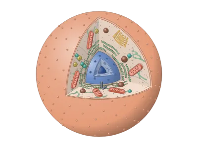 Animal cell, cut open (3D)
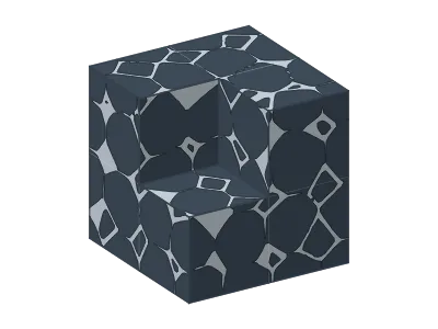 Porous solids (3D)
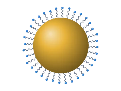 Nanoparticle
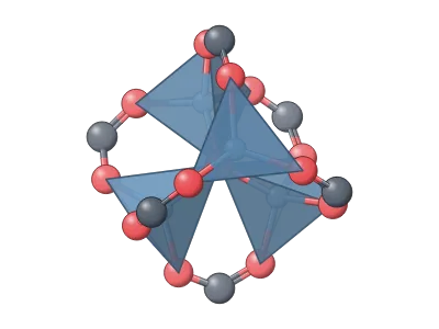 MOF building unit (SBU)
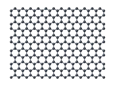 Graphene
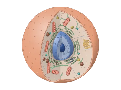 Animal cell with a wedge cut out (3D)
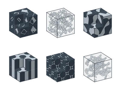 Porous solids: six kinds side by side
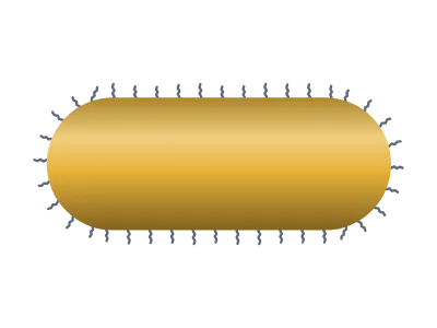 Gold nanorod
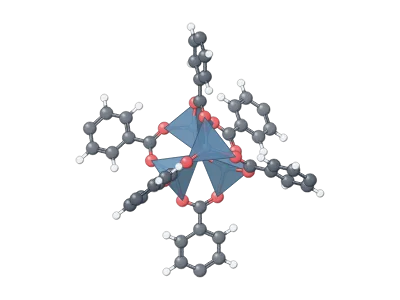 Zn₄O cluster with linkers (MOF-5)
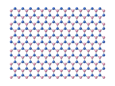 h-BN
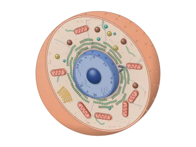 Animal cell cut in half (3D)
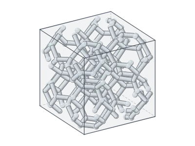 Open-cell foam (3D)
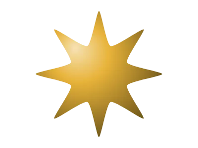 Nanostar
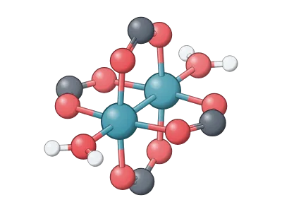 Cu paddlewheel (HKUST-1)
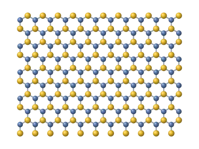 MoS₂
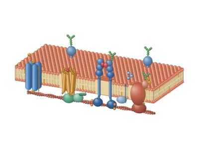 Cell membrane with receptors and channels (3D)
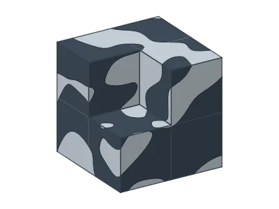 Bicontinuous porous sponge (3D)
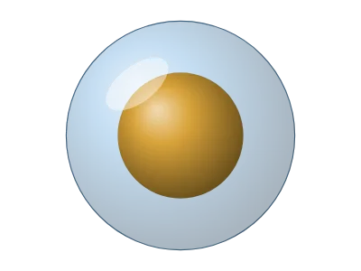 Core–shell
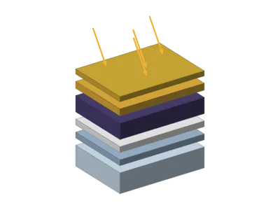 Solar cell
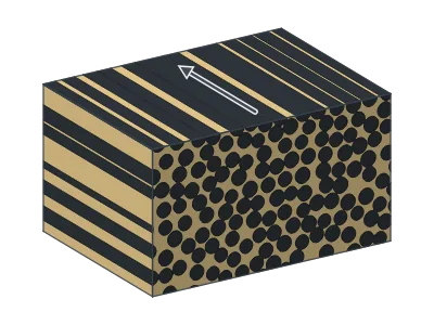 Composite microstructure (3D)
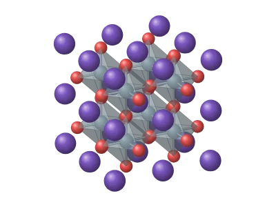
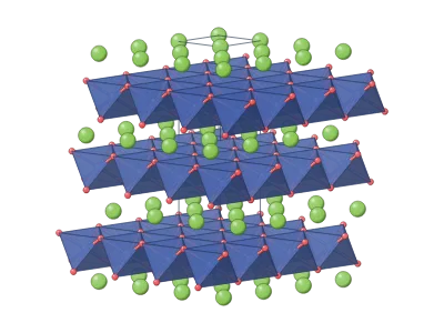 Electrode crystal
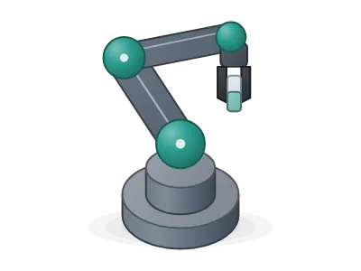 Robot arm
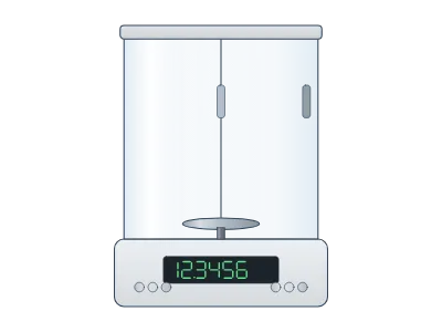 Analytical balance
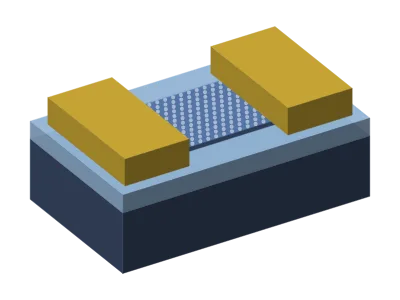 Transistor (FET)
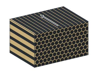 Unidirectional composite, hexagonal packing (3D)
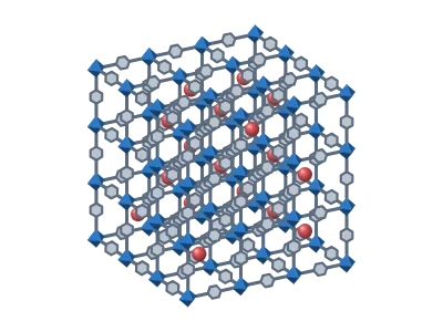
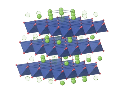 Li₀.₅CoO₂ (half charged)
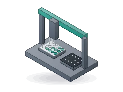 Liquid-handling robot
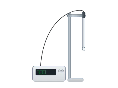 pH meter
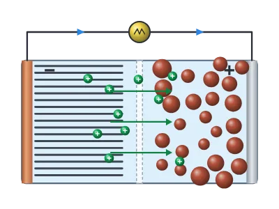 Battery
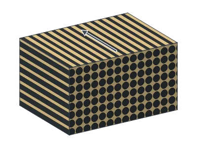 Unidirectional composite, square packing (3D)
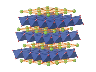 LiCoO₂ with 2D lithium planes
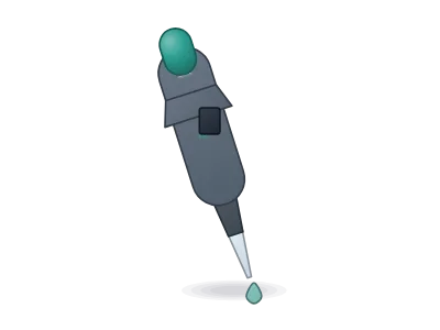 Pipette
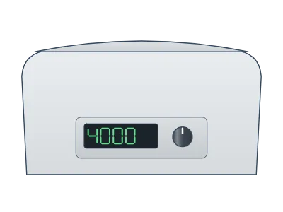 Centrifuge
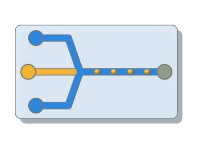 Microfluidic chip
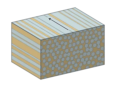 Glass-fibre composite, GFRP (3D)
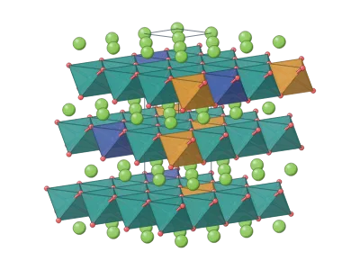 NMC811 (layered)
192 templates of real syntheses, from graphene exfoliation and CVD growth to MOFs, MXenes, Stöber silica and gold nanorods. Each one is drawn with editable layers and cites the papers it follows.
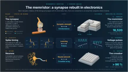 Memristors for brain-inspired computing: the synapse and its electronic twin
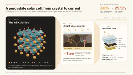 Perovskite solar cell: from crystal to device
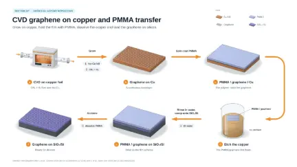 CVD graphene on copper and PMMA transfer
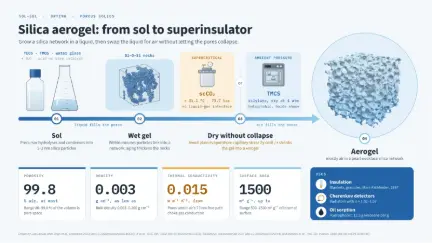 Silica aerogel: from sol to superinsulator
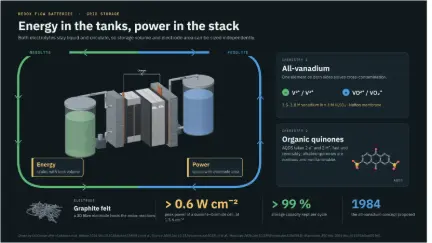 Redox flow batteries: energy in the tanks, power in the stack
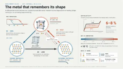 Shape-memory alloys: NiTi switches between austenite and martensite
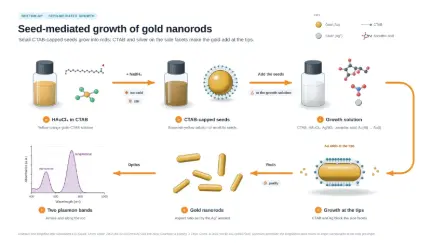 Seed-mediated growth of gold nanorods
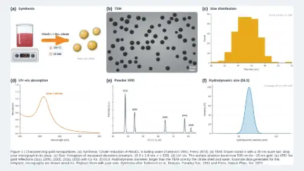 Six-panel figure: characterizing gold nanoparticles
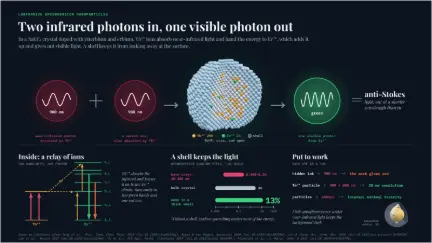 Upconversion nanoparticles: two infrared photons in, one visible photon out
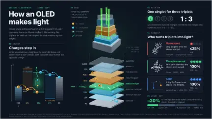 How an OLED makes light
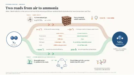 Making ammonia: Haber–Bosch on iron versus lithium-mediated electrosynthesis
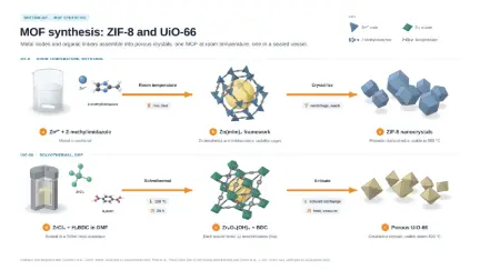 MOF synthesis: ZIF-8 and UiO-66
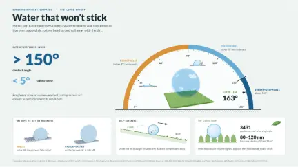 Superhydrophobic surfaces: the lotus effect, read on a protractor
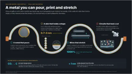 Gallium liquid metals: a metal you can pour, print and stretch
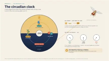 The Drosophila circadian clock
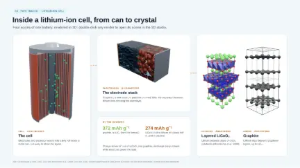 Inside a lithium-ion cell, from can to crystal (3D renders)
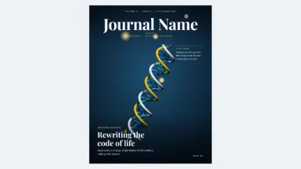 Journal cover: genome editing
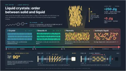 Liquid crystals: order between solid and liquid
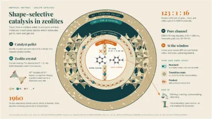 Shape-selective catalysis in zeolites: from pellet to pore window
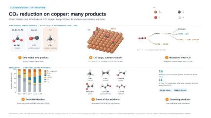 CO₂ reduction on copper: many products
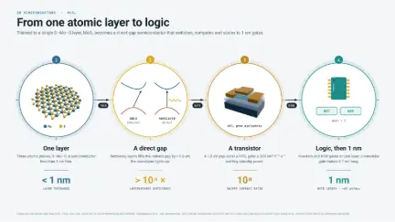 Monolayer MoS₂: from one atomic layer to logic
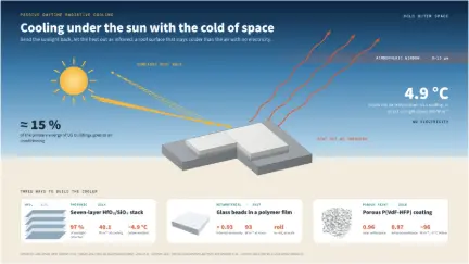 Daytime radiative cooling: cooling under the sun with the cold of space
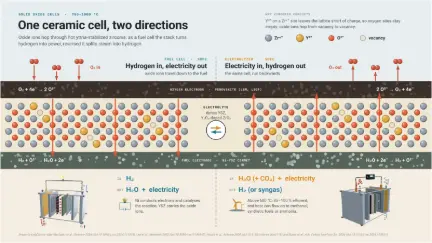 Solid oxide cells: one ceramic cell, run as a fuel cell or an electrolyzer
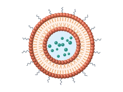
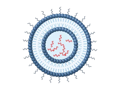
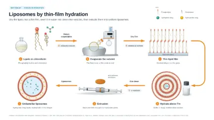 Liposomes by thin-film hydration and extrusion
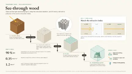 Transparent wood: take out the lignin, fill in a matching polymer
Each app does one job well, and everything it makes can go into the others. Open the ones you use as tabs: they all run in the same window.
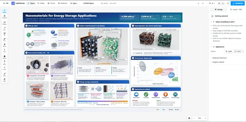 Figure editorVector figures with 500+ science objects, equations and journal-ready export.
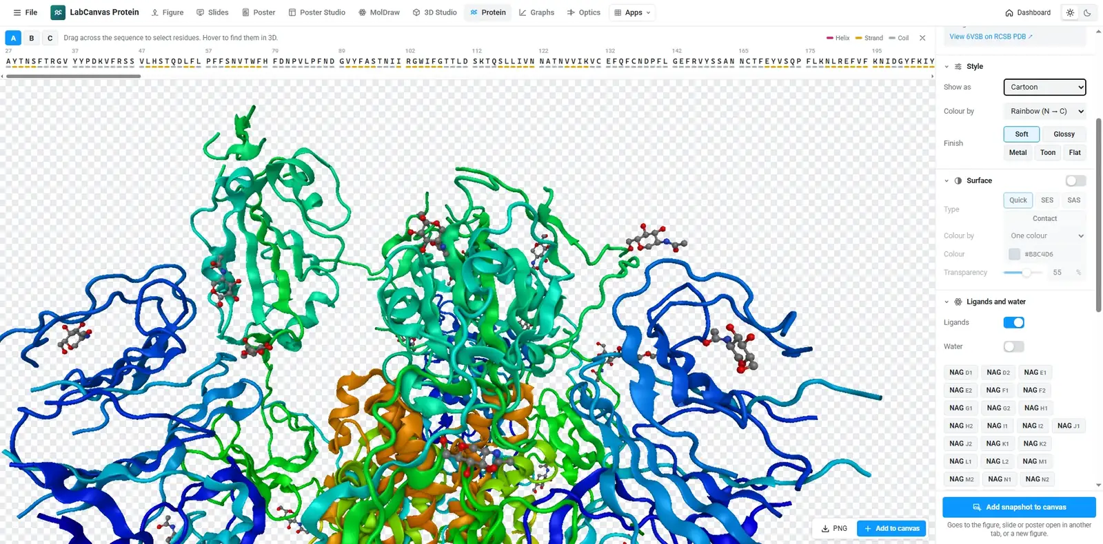
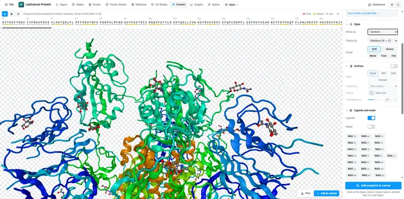 Protein viewerAny PDB entry, styled by chain, residue or ligand, snapshotted to your figure.
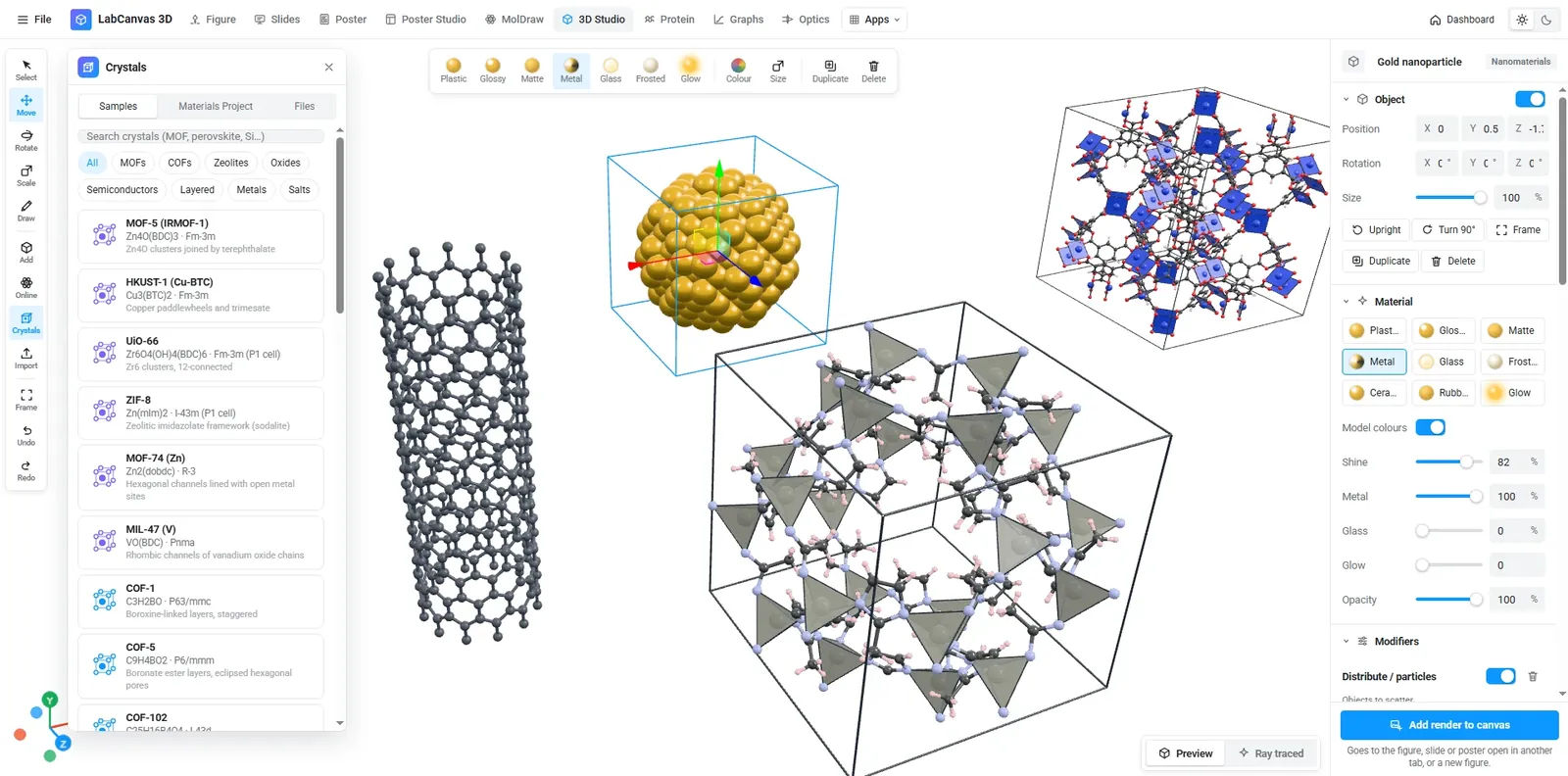
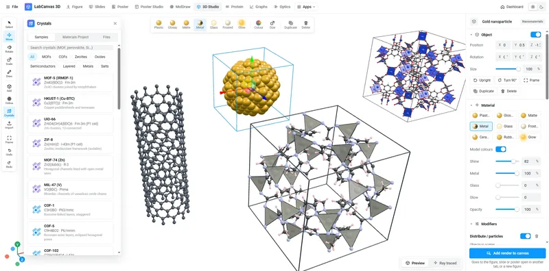 3D StudioNanomaterials, viruses, crystals and molecules, ray traced.
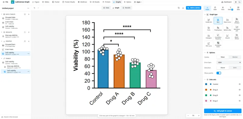 Graphs & statisticsPrism-style tables, tests and graphs that stay linked to your figure.
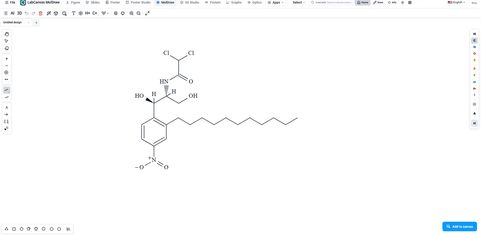
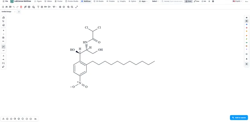 MolDrawMolecules and reactions, with a 3D view of the same structure.
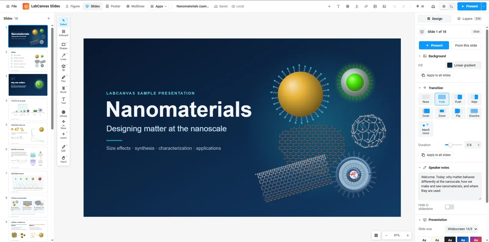
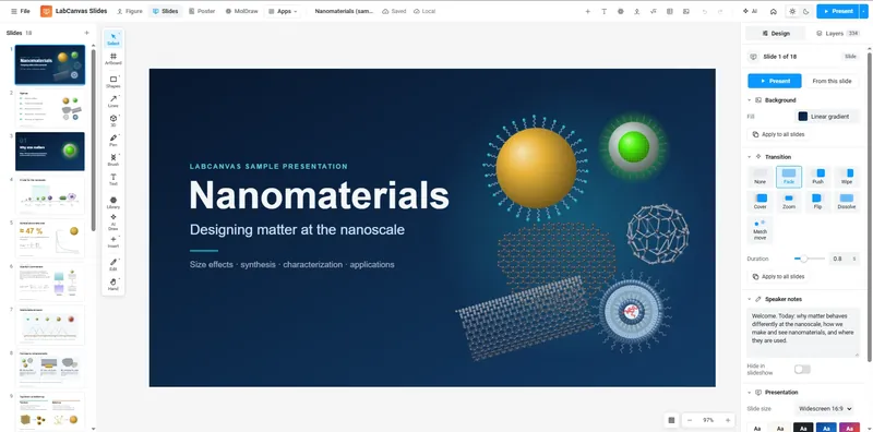 SlidesDecks built on the figure editor, with builds and match-move transitions.
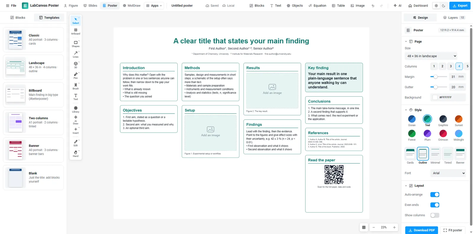
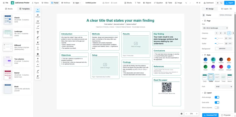 Research PosterBlocks in columns that re-flow when you move or resize them, from A0 and 48 × 36 in templates.
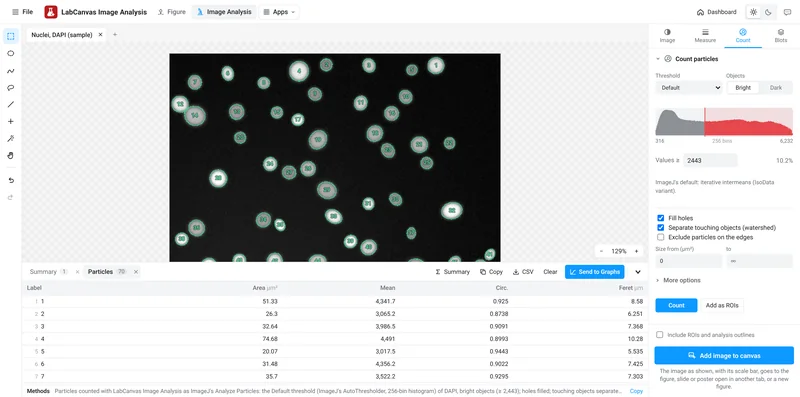 Image AnalysisBlots, cells and fluorescence, measured on the raw pixels and graphed.
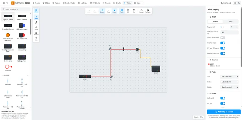 OpticsLasers, lenses and fibres on a breadboard, simulated as you build.
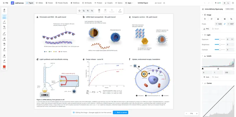 Pixel editorCrop, levels, curves and retouching, in place on the canvas.
LabCanvas Image Analysis measures TEM and SEM images of nanomaterials: nanoparticle size distributions, nanorod length and width, lattice spacing from HRTEM fringes, pore size and porosity, grain size and the lateral size of 2D flakes, in nm from the image's own scale. It opens TIFF stacks from any microscope (16- and 32-bit, hyperstacks and OME-TIFF) and measures the raw pixel values. Guided assays take you from image to results table: nuclear translocation, spots per cell, colony counts, wound healing, FRAP, calcium ΔF/F₀, particle tracking, kymographs, neurite branching, Sholl analysis and tube formation. The everyday tools sit alongside: western blot densitometry with loading-control normalisation, nuclei counting with watershed, colocalisation (Pearson, Manders, Costes), line profiles, colour deconvolution for IHC, a trainable pixel classifier, spot detection, Z projections and drift correction. Every result goes to Graphs with one click. Below, each picture is the app on its built-in sample image.
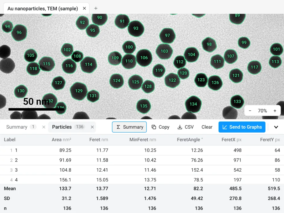 Nanoparticle size from TEM136 gold nanoparticles counted, touching ones split by the watershed: Feret diameter 13.77 ± 1.589 nm (mean ± SD)
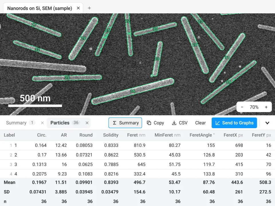 Nanorod length and width (SEM)36 nanorods (those cut by the frame left out): length 496.7 ± 154.6 nm (Feret), width 53.47 ± 10.17 nm (MinFeret), aspect ratio 11.51 ± 3.885
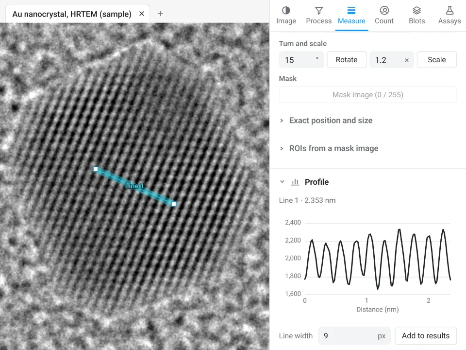 Lattice spacing from HRTEMProfile across the lattice fringes of a gold nanocrystal: 10 spacings over 2.353 nm, so d = 0.235 nm, the Au (111) spacing
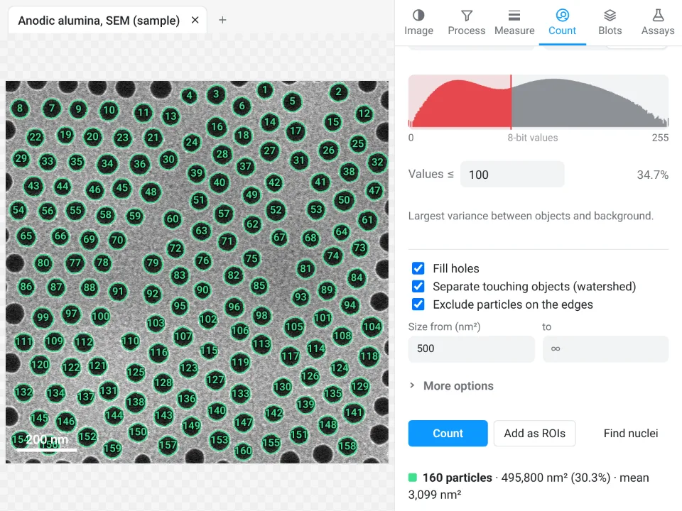 Pore size and porosity (AAO)160 pores counted (those cut by the frame left out): mean area 3,099 nm², an equivalent diameter of 62.8 nm; the pores take up 34.7% of the surface (porosity)
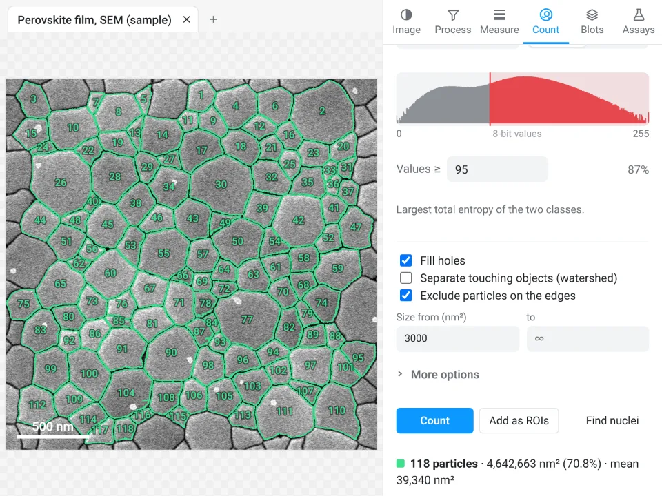 Grain size of a thin film118 grains of a perovskite film (those cut by the frame left out): mean grain area 39,340 nm², an equivalent diameter of 224 nm
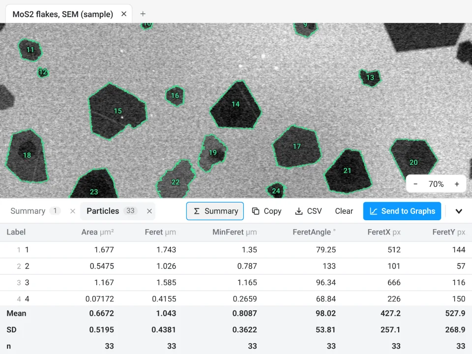 2D flake lateral size33 MoS₂ flakes (those cut by the frame left out): lateral size (Feret) from 0.3502 to 1.743 µm, 1.043 ± 0.4381 µm on average
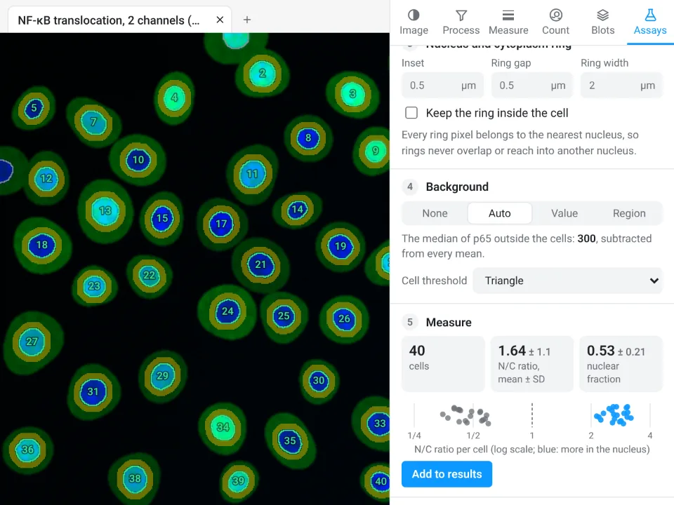 Nuclear vs cytoplasmic signal40 cells, nuclear/cytoplasmic ratio 1.64 ± 1.1, nuclear fraction 0.53 ± 0.21
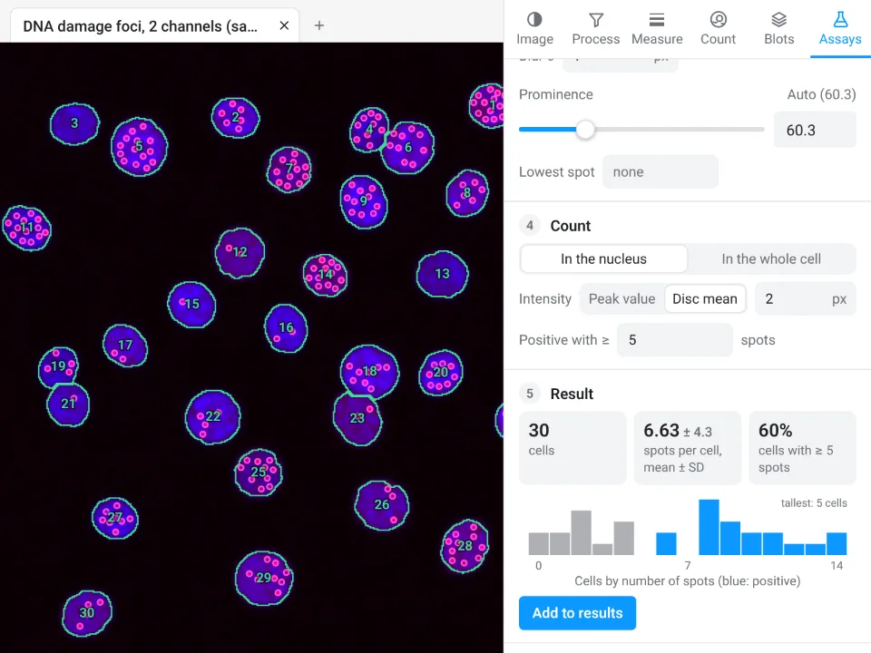 Spots per cell30 cells, 6.63 ± 4.3 spots per cell, 60% of cells with 5 or more
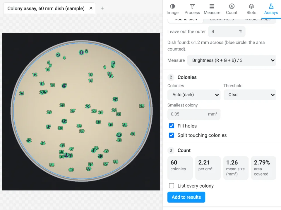 Colony counting60 colonies (2.21 per cm²), mean size 1.26 mm², 2.79% of the dish covered
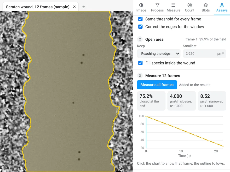 Wound healing (scratch)Scratch 75.2% closed by the last frame, closing at 4,000 µm²/h (R² 1.000)
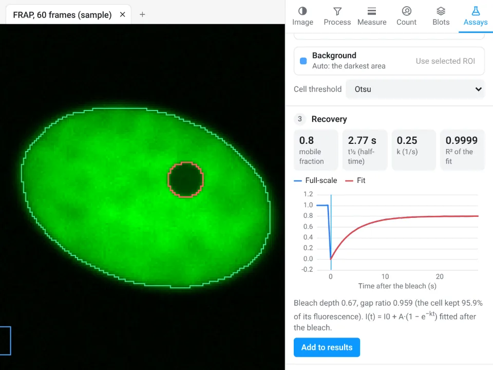 FRAP recoveryMobile fraction 0.8, recovery half-time 2.77 s, fit R² 0.9999
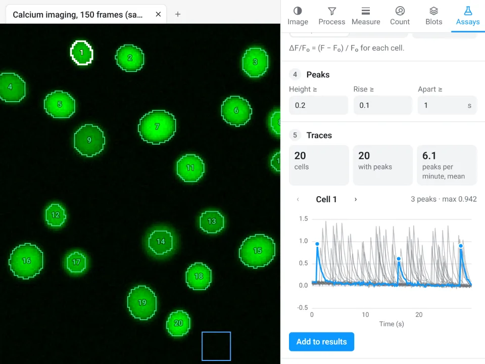 Calcium traces (ΔF/F₀)20 cells traced, 20 with peaks, 6.1 peaks per minute on average
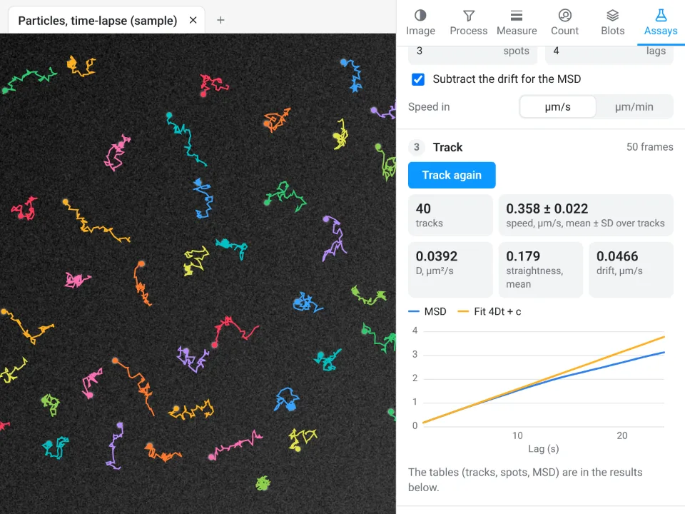 Particle and cell tracking40 tracks, speed 0.358 ± 0.022 µm/s, diffusion coefficient D 0.0392 µm²/s
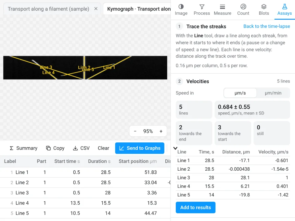 Kymograph5 particle streaks traced on the kymograph: velocities from -1.42 to 1 µm/s, speed 0.684 ± 0.55 µm/s (mean ± SD)
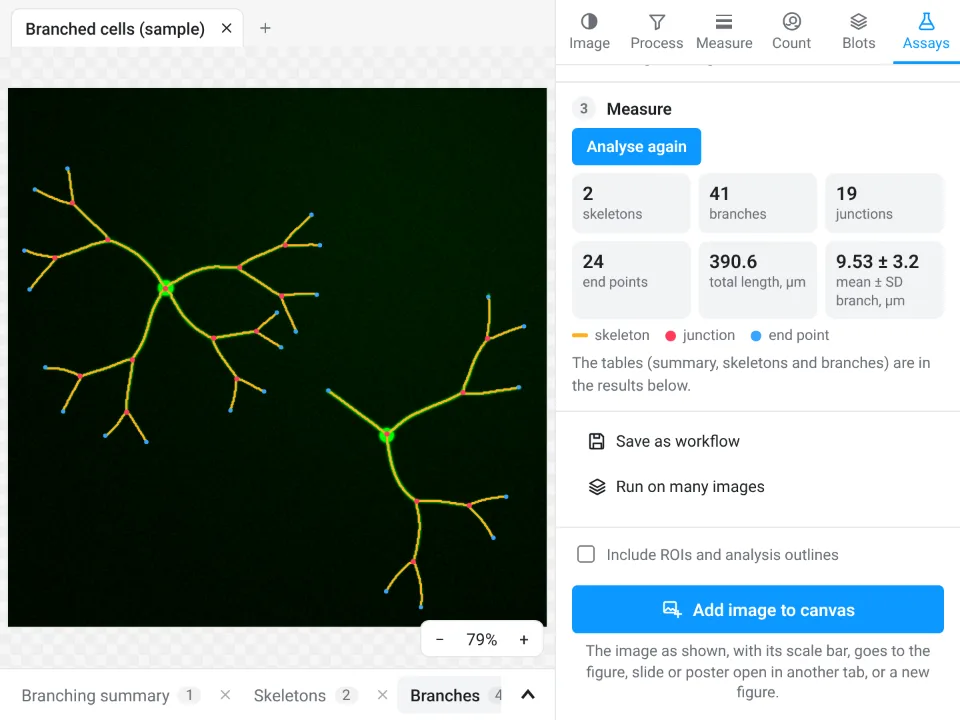 Branching and skeleton41 branches, 19 junctions and 24 end points; total length 390.6 µm
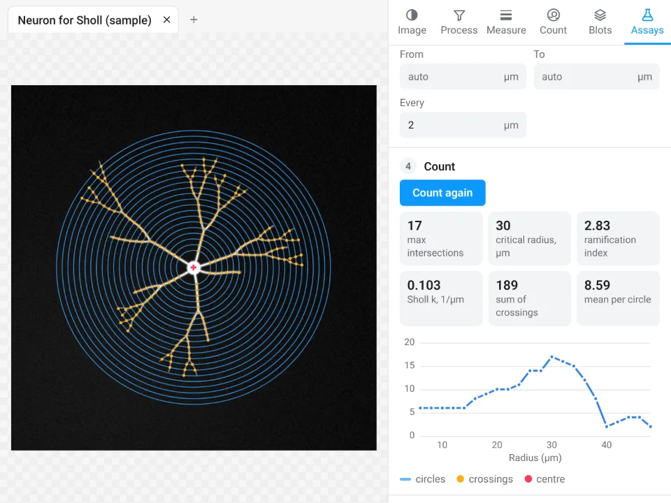 Sholl analysisUp to 17 branch crossings, on the circle 30 µm from the cell body; ramification index 2.83
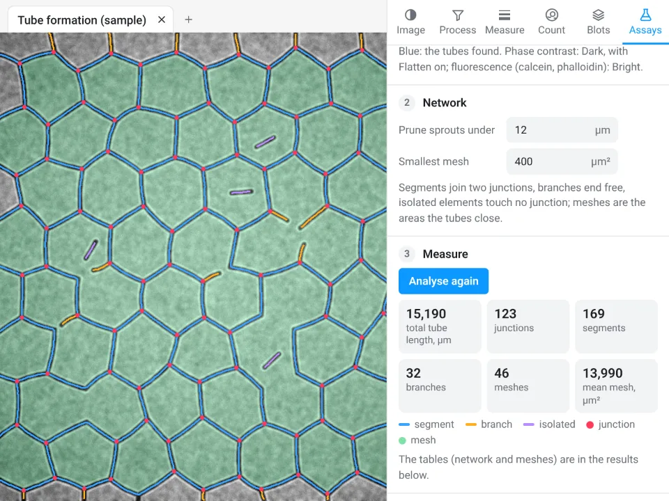 Tube formationTotal tube length 15,190 µm, 123 junctions, 169 segments, 46 meshes
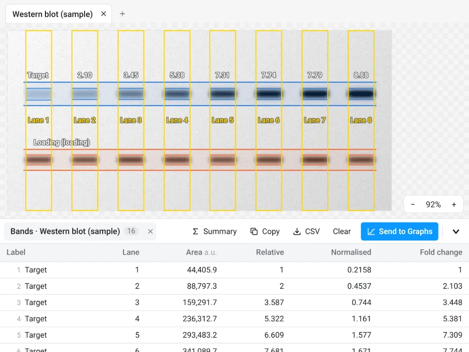 Western blot densitometry8 lanes; the target band normalised to the loading control rises from 1 (lane 1) to 8.885-fold (lane 8)
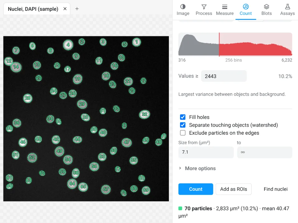 Counting nuclei70 nuclei counted (Otsu threshold, watershed to split touching ones): mean area 40.47 µm², 10.2% of the field
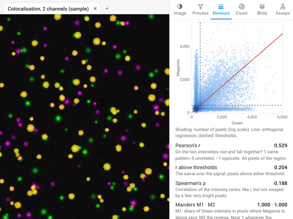 ColocalisationPearson's r 0.529; above the Costes thresholds tM1 0.219 and tM2 0.214 (7,169 colocalised pixels, in yellow)
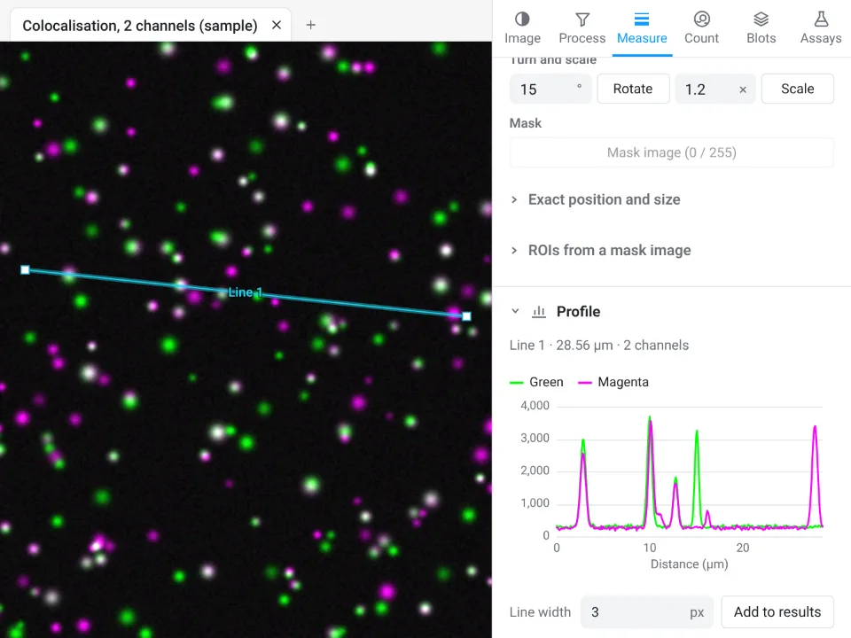 Line intensity profileGreen and magenta values along a 28.56 µm line (Line 1, 3 px wide), one curve per channel
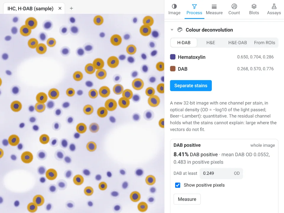 Colour deconvolution (IHC)Hematoxylin and DAB separated by colour deconvolution: 8.41% of the section DAB positive, mean DAB OD 0.0552 (0.483 in the positive pixels)
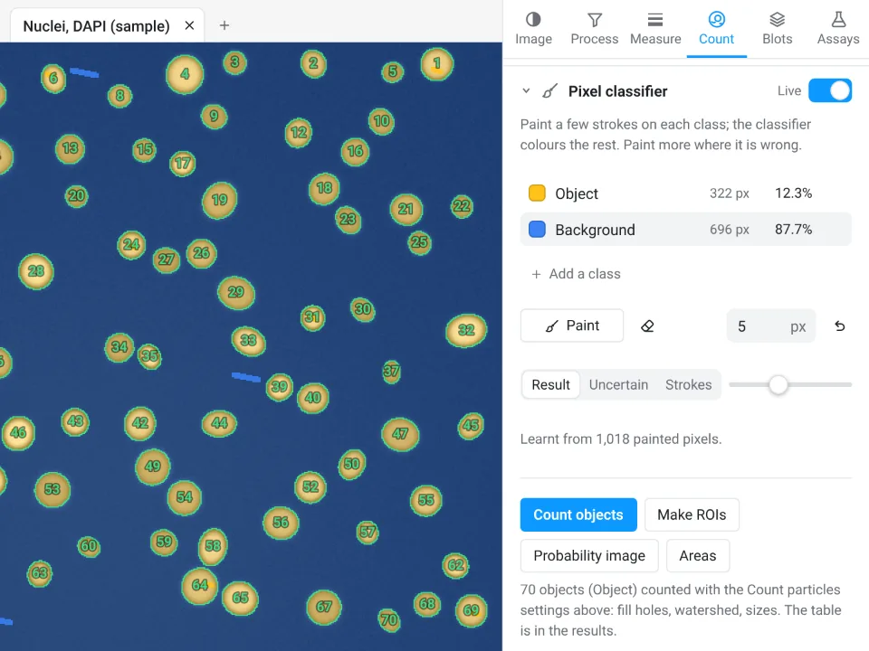 Pixel classifierTrained on 1,018 painted pixels: 70 objects counted, the Object class covering 12.3% of the image
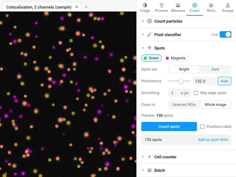 Spot detection150 spots found in the green channel, with the prominence (132.5) set automatically from the image's noise
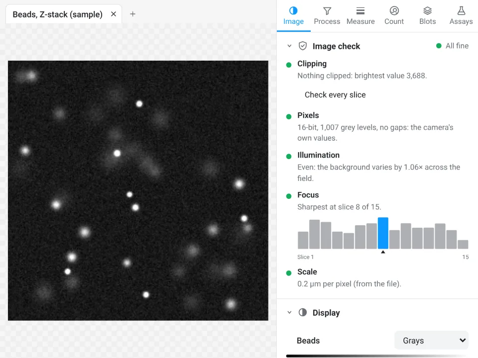 Image checkAll fine: nothing clipped (brightest value 3,688), even illumination (the background varies by 1.06×), sharpest at slice 8 of 15
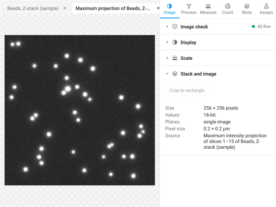 Z-stack projectionMaximum intensity projection of slices 1–15 of the bead Z-stack: the beads from every depth sharp in one 256 × 256 image
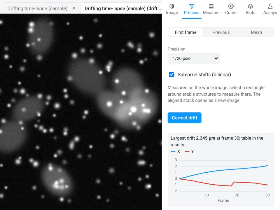 Drift correctionDrift of every frame measured against the first and corrected: largest drift 2.345 µm, at frame 30
Open Image Analysis, free How the measurements are validated
Complete A0 conference posters made in LabCanvas Research Poster: title, introduction, methods, results, conclusions, references and a QR code, with illustrations, molecules and graphs. Open one and it becomes your copy: double-click a graph to change its data, or drag a block to another column and the poster re-flows.
NMC111, NMC622 and NMC811 side by side: synthesis scheme, voltage profiles, capacity retention and why Ni-rich particles crack.
Open in Research PosterA zirconium MOF made with more and more acetic acid: synthesis, PXRD, N₂ isotherms, defect models and linkers counted by TGA.
Open in Research PosterSeed-mediated gold nanorods: growth scheme, UV–vis–NIR spectra, plasmon against aspect ratio and a TEM length histogram.
Open in Research PosterA review poster: the lattice and the Dirac cone, finding and counting layers by optical contrast and Raman, and what one layer does in devices.
Open in Research PosterThe electrolyzer and its 1.23 V, HER and OER overpotentials at 10 mA cm⁻², the hydrogen-binding volcano, and catalysts from Pt and MoS₂ edges to NiFe LDH.
Open in Research PosterThe ABX₃ crystal, n-i-p and p-i-n stacks, 3.8 % to 10.9 % in three years, more than 1.1 V from a 1.55 eV gap, and perovskite/silicon tandems.
Open in Research PosterBuilding blocks that set the net, the first boronate COFs, linkages from reversible to robust, stacking and powder patterns, and uses in CO₂ reduction and membranes.
Open in Research PosterGraphene, hBN and MoS₂, then Ti₃C₂Tₓ etched out of the MAX phase Ti₃AlC₂: its surface terminations, delamination into flakes and clay films.
Open in Research PosterWhy soluble polysulfides fade Li–S cells, three host designs (mesoporous carbon, yolk–shell, polar oxides) and the capacities and fade rates they report.
Open in Research PosterSilicon swells as it takes up lithium: the 150 nm fracture limit, nanowires, double-walled tubes, yolk–shells and pomegranates, with their cycle lives.
Open in Research PosterSulfide and garnet electrolytes, a wetting interlayer that drops interface resistance, and why voids left by stripping set the critical current.
Open in Research PosterA flow battery that keeps energy in tanks, a vitamin-derived negolyte made soluble with nicotinamide, its capacity, cycling and power.
Open in Research PosterEquiatomic fcc alloys that get stronger and tougher as they cool: twinning, the fcc-to-hcp step at 20 K, and fracture toughness across temperatures.
Open in Research PosterSingle Pt atoms on a support, how an axial Cl ligand changes their coordination, and the hydrogen-evolution activity it brings.
Open in Research PosterA layered rock-salt-derived crystal with anharmonic bonds: very low thermal conductivity, ZT along each axis and doping for high ZT over a wide range.
Open in Research PosterA quantum-dot LED stack, an interlayer that stops oxidation at the dot surface, and the efficiency and lifetime it reaches in pure blue.
Open in Research PosterOne synthesis with different co-dopants gives blue to red carbon dots: where each colour comes from, quantum yields and a two-colour probe.
Open in Research PosterWhy printed metals grow long columnar grains, and three ways out: nucleant nanoparticles, solute and ultrasound, with the grain sizes and strengths reached.
Open in Research PosterThe main things people make in LabCanvas, and the app that does each one. They run in the same window, so a render, a graph or a photo goes straight into your figure, slides or poster.
Draw figures and graphical abstracts with vector shapes, the pen and scientific brushes for DNA, membranes and proteins. Add any of 500+ science objects and change every detail with a setting.
Build nanomaterials, crystals and devices in the 3D Studio, or bring in molecules from PubChem and proteins from the PDB. Render them ray traced and drop the image into your figure.
Type or paste your data into tables, run t tests, ANOVA and curve fits, and make publication graphs with significance brackets. The results are checked against SciPy and statsmodels.
Crop micrographs and photos, set levels and curves, and retouch dust or scratches in the Pixel workspace, right on your figure, without a separate image editor.
Put your figures on slides with transitions, or lay them out on a research poster that re-flows as you edit. When you submit, export TIFF, PDF, PNG or SVG at the width and resolution the journal asks for.
Membranes, ligands, pores and lattices are parameters, not pixels. Open one in the figure editor, or turn its 3D model in the 3D Studio.
Plus equations, tables, lab glassware and scientific brushes. Browse the gallery, with the 3D models
Describe what you need, or attach a sketch, a figure or a paper. The assistant works through the same actions as the toolbar, in the figure editor, Slides, the 3D Studio and the Protein viewer.
Runs on leading models such as Claude, with monthly AI credits in every LabCanvas Pro plan. No API keys; your chats are saved to your account.
It creates real, editable layers, shows each action in the chat, and one click undoes a whole answer.
97 tools let Claude Desktop, Claude Code and other MCP clients build figures, slides, posters, graphs and 3D scenes in your open apps.
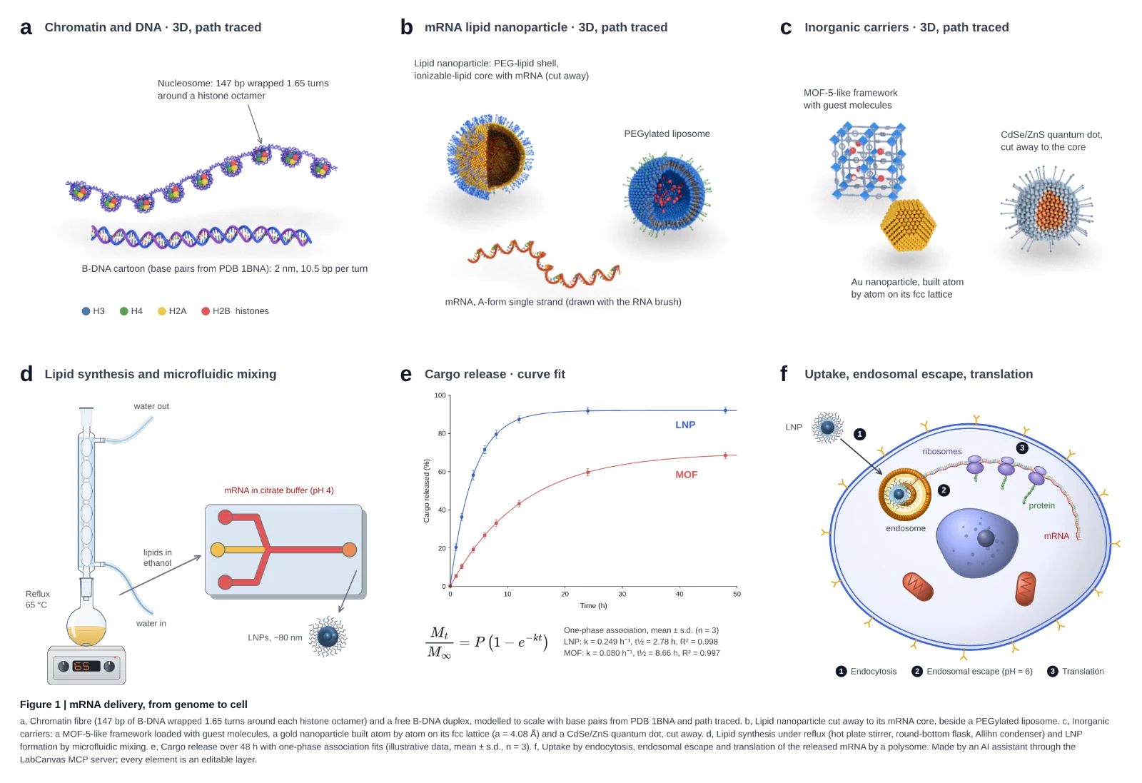
An AI assistant drove LabCanvas through its MCP server: path-traced 3D molecules, glassware assembled joint by joint, a curve fit with its equation and a cell schematic. Every panel is an editable layer.
The details that make a figure acceptable to a journal, handled by the app instead of by you.
Set the width in millimetres and the resolution (300, 600 or 1200 dpi) and export TIFF, PDF, SVG, PNG, JPEG or WebP. Files carry their DPI, so the size is right when the journal opens them.
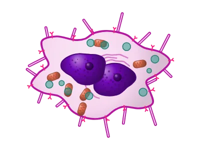
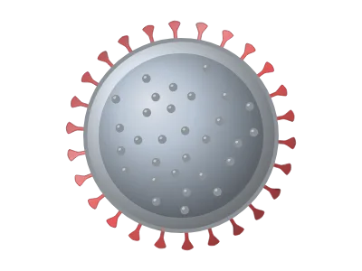
Liposomes, cancer cells, viruses, nanoparticles, crystals, hydrogels, devices and lab instruments: drawn by generators, so every detail is a setting.
Equations typeset by MathJax into vector outlines, and editable tables with scientific (booktabs) styles.
Flasks, condensers, still heads, adapters, funnels, burettes, stands, hot plates, furnaces and gloveboxes at real proportions. Pieces snap onto each other’s joints and tubing follows them, so a distillation setup stays assembled as you move it.
Import compounds from PubChem and structures from the RCSB PDB; show them as cartoons, surfaces or ball-and-stick.
Prism-style analyses whose results are validated against SciPy, statsmodels, lifelines and R in more than 42,000 automated checks.
Drag a block between two others or into another column and the poster re-stacks; resize it and the text re-flows. A0 and 48 × 36 in templates, themes, QR codes and a print-ready vector PDF.
Designs autosave in your browser and, if you choose, to your own private cloud folder so you can open them on any computer. Nothing is public, and nobody else can open your work.
Anything else? Write to our team.
LabCanvas is a browser-based workspace for scientific visuals. It combines a vector figure editor, a presentation maker, a research poster designer, a 3D studio, a protein structure viewer and a graphing and statistics app, with journal-ready export and an AI assistant.
Every app is free to use with an account, with up to 3 designs; downloading and exporting are part of LabCanvas Pro, paid monthly or yearly (see the pricing page for the price in your country). LabCanvas Pro also gives unlimited designs and a monthly allowance of AI credits for the assistant. Choose monthly or yearly and pay securely through Dodo Payments; cancel any time. The website and the free tools at /tools need no account and no payment.
In your browser’s storage (IndexedDB) on your own device, and, with cloud saving on (the default for new designs), in your own private folder in LabCanvas cloud, so they open on any computer. You can switch cloud saving off for any design, and File › Save a copy keeps a portable .labcanvas file.
Yes. Share a figure, presentation or poster from its Share button, by a link or with people by e-mail, as view, comment or edit. Everyone who has it open sees the others’ changes as they are made, with their pointers and what they have selected, and the design saves itself a few seconds after the last change. It works on the free plan too.
PNG, JPEG, WebP, TIFF, PDF and SVG. You set the physical width in millimetres and the resolution (for example 300, 600 or 1200 dpi); PNG and TIFF files record their DPI. Presentations export as one vector PDF.
Yes. LabCanvas Research Poster starts from a template (A0 or A1 portrait, 48 × 36 in landscape, a billboard-style #betterposter layout and more) built from blocks: title, sections, figures, a key finding, a big number, references and a QR code. Drag a block to another column or between two others and the columns re-stack; resize it and the text re-flows. Themes restyle every block at once, and the poster exports as a vector PDF at its exact printed size.
Yes. Objects › Equation typesets LaTeX, including AMS environments and chemistry with \ce{…}, into vector outlines that stay sharp in PDF and SVG. Double-click an equation to edit its LaTeX later.
Open the Protein viewer, enter a PDB ID such as 1CRN or 4HHB, pick a style (cartoon, surface, ball-and-stick…) and a colouring, select residues on the sequence bar to highlight or restyle them, then download a PNG or add it to your figure.
The assistant runs on leading models such as Anthropic Claude, chosen and set up by LabCanvas: there is no API key to paste. Each LabCanvas Pro plan includes monthly AI credits; you can attach images and PDFs to your messages, and your chats are saved to your account. The assistant edits through the same actions as the toolbar, so every change can be undone.
LabCanvas includes a Model Context Protocol (MCP) server with 97 tools, so AI agents such as Claude Desktop or Claude Code can create and edit figures, slides, posters, graphs, 3D scenes and optical setups in your open LabCanvas apps.
Yes. The figure editor, Slides, the 3D Studio, the Protein viewer and the Graph app can each be installed from the browser and opened like desktop apps.
Every app is free to start in your browser, with up to 3 designs. LabCanvas Pro adds downloads, unlimited designs and the AI assistant.
Start free See pricing