Free account · save your work, full figure editorSign up free

ELISA standard curve calculator with 4PL curve fitting

Q: What is a 4PL curve?

A four-parameter logistic curve: y = Bottom + fracTop - Bottom1 + (EC₅₀ / x)^Hill Bottom and Top are the flat ends of the S-shaped curve, EC50 is the concentration halfway between them, and the Hill slope sets how steep it is. It fits the whole standard range, not only the straight middle part.

Enter your standards (concentration and OD, with replicates) and your samples’ ODs and dilution factors. The calculator fits a four-parameter logistic (4PL) standard curve, or a linear or log-log line, subtracts the blank, and calculates each sample’s concentration, flagging values outside the standard range. It works for sandwich and competitive ELISAs. You get R², the fitted parameters, a chart and a CSV.

What it does: Fits an ELISA standard curve (4PL, linear or log-log) to your standards’ ODs and converts sample ODs into concentrations, with blank subtraction and dilution factors.
Formula: $\begin{aligned} &\text{4PL: } y = \mathrm{Bottom} + \frac{\mathrm{Top} - \mathrm{Bottom}}{1 + (\mathrm{EC}_{50} / x)^{\mathrm{Hill}}} \\ &\text{inverse: } x = \mathrm{EC}_{50} \\ &\quad {}\times \left(\frac{\mathrm{Top} - \mathrm{Bottom}}{y - \mathrm{Bottom}} - 1\right)^{-1/\mathrm{Hill}} \end{aligned}$
Example: With Bottom 0.024, Top 2.865, EC50 280 pg/mL and Hill 1.19, a blank-corrected OD of 0.885 reads 139 pg/mL; diluted 1:2, the sample holds 277 pg/mL.

Last updated 8 November 2026

FreeNo sign-upRuns in your browserData analysis

Loading ELISA standard curve calculator…

At a glance

ELISA standard curve calculator at a glance
Models	4PL (recommended), linear and log–log
Fit	Levenberg–Marquardt, the same fitter as the LabCanvas Graphs app, validated against SciPy
Handles	Replicates with CV %, blank subtraction, dilution factors
Flags	Samples outside the standard range
Output	Standard curve (PNG, SVG) and CSV
Runs in	Your web browser; nothing is uploaded
Price	Free, no account needed

What it does

How to use the ELISA standard curve calculator

Enter the standardsConcentration and up to three OD replicates per standard; paste from a plate-reader export or type them in.
Enter the samplesName, OD replicates and dilution factor for each unknown.
Fit and readKeep the 4PL model unless your kit says otherwise; read the concentrations and check the range flags, then export.

How it works

$\text{4PL: } y = \mathrm{Bottom} + \frac{\mathrm{Top} - \mathrm{Bottom}}{1 + (\mathrm{EC}_{50} / x)^{\mathrm{Hill}}}$ $x = \mathrm{EC}_{50} \times \left(\frac{\mathrm{Top} - \mathrm{Bottom}}{y - \mathrm{Bottom}} - 1\right)^{-1/\mathrm{Hill}}$

The 4PL curve is fitted by Levenberg–Marquardt least squares on log concentration (the same fitter as the LabCanvas Graphs app, validated against SciPy), using every replicate as its own point. The mean OD of each unknown, minus the blank, is converted back to a concentration with the inverse of the curve and multiplied by its dilution factor. Values above the top standard or below the lowest are flagged, because extrapolated concentrations are unreliable.

Worked example: an ELISA standard curve with a 4PL fit

The calculator’s example data, step by step: a sandwich ELISA with a two-fold standard series from 1000 to 15.6 pg/mL, three OD readings per standard and a zero standard (blank).

Subtract the blank. The zero standard reads 0.062, 0.058 and 0.065; its mean, 0.062, is subtracted from every OD.
Fit the 4PL curve to the 21 standard readings (each replicate is its own point), on log concentration. Result: Bottom = 0.024, Top = 2.865, EC50 = 280 pg/mL, Hill slope = 1.19, R² = 0.9997.
Check the curve by back-calculating the standards. Each standard’s mean OD is read back through the curve; recoveries within about 80–120 % (75–125 % at the lowest and highest standards) mean the curve describes the data.

Back-calculated standards (example data)
Nominal (pg/mL)	Mean OD − blank	Back-calculated (pg/mL)	Recovery
1000	2.349	995.5	99.6 %
500	1.921	503.8	100.8 %
250	1.345	248.6	99.4 %
125	0.813	124.9	99.9 %
62.5	0.437	62.8	100.6 %
31.25	0.224	31.7	101.5 %
15.6	0.110	15.1	96.6 %

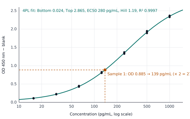
ELISA 4PL standard curve: seven standards from 15.6 to 1000 pg/mL on a log axis with the fitted S-shaped curve; sample 1 at OD 0.885 reads 139 pg/mL — The 4PL standard curve of the example data, with sample 1 read off the curve.

Read the samples. Sample 1 has a mean OD of 0.947, or 0.885 after the blank. Inverting the curve: $\begin{aligned} x &= 280 \times \Bigl(\tfrac{2.865 - 0.024}{0.885 - 0.024} - 1\Bigr)^{-1/1.19} \\ &= 139\ \mathrm{pg/mL} \end{aligned}$ in the well.
Apply the dilution. Sample 1 was diluted 1:2, so it contains $139 \times 2 = \mathbf{277\ pg/mL}$ . Sample 2 (OD 1.443 after the blank, diluted 1:10) reads 279 pg/mL in the well, or 2794 pg/mL; sample 3 (OD 0.175, undiluted) reads 24.7 pg/mL.

4PL or 5PL?

The 4PL curve is symmetric around its midpoint (the EC50) when concentration is on a log scale. The five-parameter logistic (5PL) adds an asymmetry factor $S$ : $y = \mathrm{Bottom} + \frac{\mathrm{Top} - \mathrm{Bottom}}{\left(1 + (\mathrm{EC}_{50} / x)^{\mathrm{Hill}}\right)^{S}}$ and $S = 1$ gives the 4PL again.

Use the 4PL for most ELISAs. It is the accepted reference model for ligand-binding assay calibration curves, and it is what most kit inserts ask for (Findlay & Dillard, AAPS J 2007).
Consider the 5PL when the curve is clearly asymmetric: one end bends more sharply than the other, and standards near the top or the bottom back-calculate consistently high or low with the 4PL even though the replicates agree. With asymmetric data the 5PL can give much more accurate concentrations than the 4PL (Gottschalk & Dunn, Anal Biochem 2005).
The 5PL needs more data. With an extra parameter it needs well-spread standards, including points on both flat ends, or the fit becomes unstable. With seven or eight standards and a symmetric-looking curve, the 4PL is usually the better choice.

This calculator fits the 4PL. The back-calculated recoveries in its results show whether a 4PL describes your standards well; if the end standards recover poorly in a consistent direction, try a 5PL fit in your plate reader’s software.

Frequently asked questions

How do you make an ELISA standard curve?

Run a dilution series of the standard (often two-fold, 6 to 8 points) and a zero standard on the same plate as the samples. Subtract the mean of the zero standard from every OD, plot OD against concentration on a log axis and fit a 4PL curve. Read each sample’s concentration from the curve and multiply by its dilution factor; samples outside the standard range are diluted and re-run.

What is the difference between 4PL and 5PL?

The 5PL adds an asymmetry parameter to the 4PL. The 4PL is symmetric on a log concentration scale and is the standard for most ELISAs; the 5PL fits curves with one end bending more sharply than the other, but needs well-spread standards on both flat ends to fit reliably.

Which curve fit should I use for ELISA?

The four-parameter logistic (4PL) is the standard for sandwich and competitive ELISAs because it follows the S-shaped response, including the flat ends. Use linear only if the kit specifies it and your standards are in the linear range.

What is a 4PL curve?

A four-parameter logistic curve: $y = \mathrm{Bottom} + \frac{\mathrm{Top} - \mathrm{Bottom}}{1 + (\mathrm{EC}_{50} / x)^{\mathrm{Hill}}}$ Bottom and Top are the flat ends of the S-shaped curve, EC50 is the concentration halfway between them, and the Hill slope sets how steep it is. It fits the whole standard range, not only the straight middle part.

Does it work for competitive ELISA kits, such as cortisol or corticosterone?

Yes. In a competitive ELISA, the usual format for small molecules such as steroid hormones, the OD falls as the concentration rises; the 4PL fit follows a falling curve as well as a rising one. The zero standard is then the maximum signal (B0) rather than a blank, so you may switch off “Subtract the zero standard” to keep the chart in measured ODs; the 4PL concentrations are the same either way.

What is a good R² for an ELISA standard curve?

Usually 0.99 or higher for a 4PL fit. Also check that standards back-calculate to within about 80–120 % of their nominal values and that replicate CVs are under about 15–20 %.

What should I do with samples above the top standard?

Dilute them further and re-run them. Concentrations extrapolated beyond the standard range are not reliable.

Should I subtract the blank?

For a sandwich ELISA, yes, if the kit includes a zero standard or blank wells: it removes background signal. The calculator subtracts the mean of the zero standard when the option is on. In a competitive ELISA the zero standard is the maximum signal, not a blank (see above).

How do dilution factors work?

If you diluted a sample 1:10 before the assay, enter 10: the concentration read from the curve is multiplied by 10 to give the original sample’s concentration.

Plot and report the standard curve

The LabCanvas Graph app fits the 4PL standard curve, reads unknowns off it with 95% confidence intervals and draws a publication-ready graph. It opens with a worked ELISA example you can replace with your data.

Open the ELISA graph