LabCanvas Image Analysis: measure microscopy images, western blots and gels in your browser
How to measure images in LabCanvas Image Analysis: guided assays (nuclear translocation, spots per cell, wound healing, FRAP, calcium, tracking, branching), western blots with a ladder and total-protein normalisation, cell counting with a trainable classifier, ROIs with ImageJ definitions, on the raw pixel values, with results sent to Graphs.
Contents
LabCanvas Image Analysis measures microscope images, western blots and gels in the browser, on their raw pixel values, with the measurement definitions of ImageJ. Guided assays take common experiments from image to table in a few steps. Results go straight to Graphs for statistics, and the images, with their scale bars, go to a figure. Every number is checked against independent software in more than 4,000 automated tests (how it is validated).
What it is for
- Fluorescence and brightfield images: intensity, area and integrated density of cells or regions, in calibrated units.
- Cell assays: nuclear vs cytoplasmic signal, spots per cell, colony counts, wound healing, FRAP recovery and calcium traces.
- Western blots and gels: band densitometry with background correction, a molecular-weight ladder and normalisation to a loading control or total protein.
- Counting and segmentation: nuclei, cells, colonies, spots or particles, by threshold, by a classifier you train with a few brush strokes, or by clicking.
- Structures and motion: branching and skeletons, Sholl analysis, tube formation, kymographs and particle tracking.
Open an image, and check it
Open a TIFF from the microscope, drop it on the window or paste it. Stacks, 16-bit and 32-bit images, ImageJ hyperstacks, OME-TIFF and BigTIFF open with their channels, slices, frames and pixel size. The Image tab starts with an image check: it warns when pixels are clipped at the camera's maximum, when the file was compressed or processed before saving, when the illumination is uneven or a slice is out of focus, and when open images cannot be compared fairly. It then sets how each channel is shown (colour, brightness and contrast with its histogram, a colour scale bar for false-colour images), which never changes the values that are measured. If the file has no scale, draw a line along a scale bar or micrometer and type the length it spans.
Guided assays
The Assays tab is a gallery of common measurements. Each opens as a few numbered steps with defaults that work in one click, shows its result on the image as you change a setting, and offers a sample image to try it on:
- Nuclear vs cytoplasmic signal: finds the nuclei, draws a cytoplasm ring around each (rings never overlap a neighbour) and gives the signal in each and their ratio, for NF-κB, YAP or TFEB translocation.
- Spots per cell: counts foci or puncta in each nucleus or cell, with their intensity and the share of cells above a number you choose.
- Colony counting: finds the dish, splits touching colonies and gives their number, sizes and the area covered.
- Wound healing: the open area and width of a scratch in every frame, % closure and the closure rate.
- FRAP recovery: bleached, reference and background regions found automatically, double normalisation, and the fitted mobile fraction and half-time.
- Calcium traces: ΔF/F₀ for every cell over time, with its peaks.
- Tracking, kymographs, branching and skeleton, Sholl analysis and tube formation for movement and structures.
Save as workflow keeps an assay's settings; a saved workflow runs on every open image or on a set of files, and the results collect in one table.
Measure regions
Draw rectangles, ovals, polygons, freehand shapes, lines or points. The Measure tab lists them; Measure adds a row per region: area, mean, standard deviation, min and max, median, integrated density, centroid, perimeter, shape descriptors, a fitted ellipse and Feret's diameter, as chosen. ROI tools combine, intersect or subtract regions, enlarge or shrink them by an exact distance, make rings, convex hulls, fitted circles and ellipses, and turn masks into regions. ImageJ ROI sets (RoiSet.zip) open and save, so regions move between LabCanvas and Fiji.
Quantify a western blot
In the Blots tab, Find lanes places a rectangle on each lane and Find bands proposes the band rows across lanes. Each band is integrated above a baseline drawn under it, as with ImageJ's gel analyser. Mark the ladder lane and type its sizes to read each band's molecular weight; normalise to a loading-control band or to the whole lane of a total-protein stain (Ponceau S, stain-free); smiling lanes are aligned before bands are matched. The table gives every band's density, its normalised value and the fold change against a reference lane.
Count cells, spots and particles
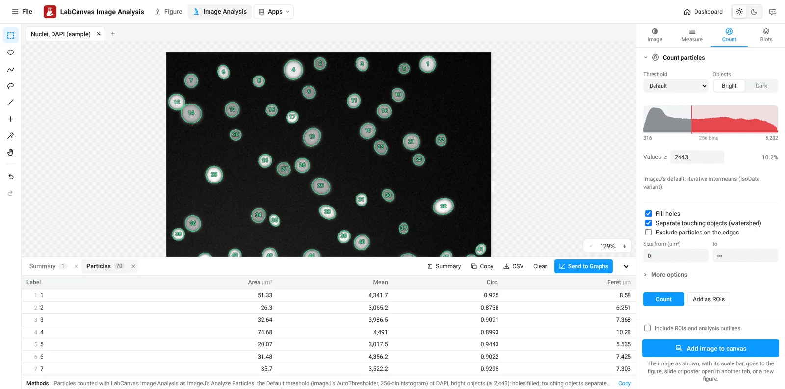
In the Count tab, choose an automatic threshold method (Otsu, Li, Triangle and ImageJ's others), watch the preview, and separate touching nuclei with watershed; Find nuclei does it in one click. When a threshold cannot separate what you want, the pixel classifier learns from a few brush strokes on each class and colours the rest; paint more where it is wrong. Spots counts maxima above a prominence you set, per cell or over the image, and the cell counter counts by clicking, in categories. Batch runs the same settings on many images.
Process, stacks and time-lapse
The Process tab subtracts background with a rolling ball, filters, enhances local contrast (CLAHE), removes noise and outliers, makes and edits binary masks, divides one channel by another for ratio images, corrects drift and separates histology stains (H-DAB, H&E) into their amounts. Each step is undoable and can open as a new image. Stacks play through their slices or frames, show orthogonal views and reslice along a line. Colocalisation gives Pearson's and Manders' coefficients with Costes' automatic thresholds.
From numbers to figures
- Send to Graphs turns a results table into a Graphs data table with a graph: one data set per image (for example control and treated), or an XY table for profiles, time series and MSD curves. Sending again updates the same table.
- Copy pastes the table into Excel; CSV saves it. Each table carries a methods sentence for the paper.
- Add image to canvas places the image as shown, with its scale bar (and its ROIs and outlines, if you tick that), in the figure, slide or poster open in another tab. Each channel and the merge sends them as separate pictures, side by side, for a panel layout in the Figure editor.
- Save project (Ctrl+S) keeps every image, ROI and results table in one .lcanalysis file to carry on later or share.
- In the Figure editor, right-click an image and choose Measure in Image Analysis to open it here (measure the original file from the instrument when you can).
Good practice
- Measure the original file from the instrument, not a picture exported for a figure: JPEG compression and figure adjustments change pixel values. The image check flags both.
- Keep acquisition settings the same for images you compare, avoid clipped pixels, and measure them with the same settings (saved workflows and Batch help).
- Contrast enhancement and denoising are for seeing and segmenting; measure intensities on the original image.
- For blots, stay within the linear range of the detection and normalise to a loading control or total protein.
Frequently asked questions
Is LabCanvas Image Analysis an ImageJ or Fiji alternative?
For everyday lab image analysis, yes: regions of interest with ImageJ's measurement definitions, western blot densitometry, cell and spot counting, colocalisation, processing, stacks, and guided assays for translocation, foci, wound healing, FRAP, calcium imaging, tracking and branching, in the browser with nothing to install. Fiji's plugin ecosystem is larger: 3D object analysis, deep-learning segmentation such as StarDist or Cellpose, and every vendor file format are not covered.
Are measurements made on the raw pixel values?
Yes. A 16-bit or 32-bit image keeps its values; brightness, contrast and colours change only how it is shown. Measurements, thresholds, assays and blot densities always read the original values, and the image check warns when the data are clipped, lossy or were processed before saving.
How accurate is it?
Every area is checked against independent software (scikit-image, SciPy, NumPy, scikit-learn, tifffile, roifile, trackpy) and against images with known answers, in more than 4,000 automated checks that must pass before each release. The image analysis validation page lists them with their tolerances.
Which files can I open?
TIFF, including multi-page stacks, 16-bit and 32-bit images, ImageJ hyperstacks, OME-TIFF and BigTIFF with their pixel size and channels, plus PNG, JPEG, WebP, GIF and BMP, ImageJ ROI sets (RoiSet.zip, .roi) and LabCanvas projects (.lcanalysis). Vendor files such as .czi, .nd2 and .lif need to be saved as TIFF (OME-TIFF keeps the scale) from the microscope software or Fiji first.
Can I run the same analysis on many images?
Yes. Every assay can be saved as a workflow with its settings, and run on all open images or on a set of files, which are opened one at a time; the results collect in one table, one row per image or per cell. Counting has its own Batch section.
How do I quantify a western blot?
Open the image, go to the Blots tab, click Find lanes and Find bands, and choose what to normalise to: a loading-control band or a total-protein stain image. Mark the ladder lane and type its sizes to get each band's molecular weight. The table gives each band's background-corrected density, its normalised value and the fold change against a reference lane.
Try it in LabCanvas
Every app is free to start in your browser. Create an account and begin.
Start Image Analysis free in your browserKeep reading
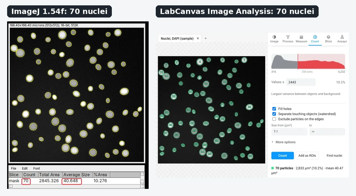
ImageJ vs LabCanvas Image Analysis: an honest comparison
ImageJ/Fiji or LabCanvas Image Analysis? Six everyday jobs done in both, six newer ones (macros, vendor files, 3D, StarDist, big images) and which to use.
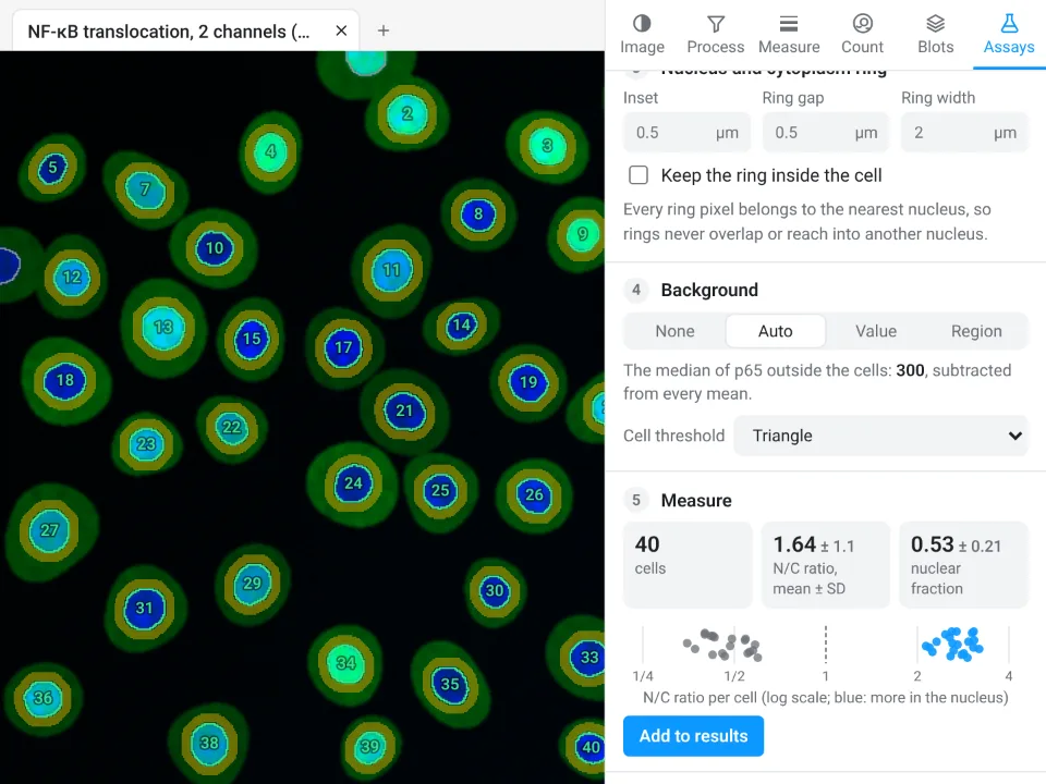
Image Analysis in LabCanvas: a complete guide to every tool and setting, with examples
Every tool in LabCanvas Image Analysis, tab by tab, with its settings and a real example: image check, display and scale, stacks and Z projection, background subtraction, filters, thresholds and binary operations, ROIs and Set measurements, Analyze Particles, a pixel classifier, spots, cell counter, western blot densitometry, colocalisation, colour deconvolution and eleven guided assays.
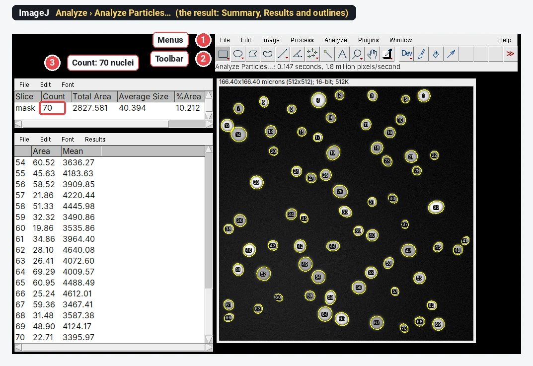
How to use ImageJ: a beginner's tutorial for the 10 everyday jobs (2026)
How to use ImageJ and Fiji: get started, open an image, then 10 everyday jobs (scale, measure, threshold, count, background, blots) with exact menu paths.