Image Analysis in LabCanvas: a complete guide to every tool and setting, with examples
Every tool in LabCanvas Image Analysis, tab by tab, with its settings and a real example: image check, display and scale, stacks and Z projection, background subtraction, filters, thresholds and binary operations, ROIs and Set measurements, Analyze Particles, a pixel classifier, spots, cell counter, western blot densitometry, colocalisation, colour deconvolution and eleven guided assays.
Contents
LabCanvas Image Analysis measures microscope images, western blots and gels in the browser, on the raw pixel values. If you have measured images on the desktop before, you will recognise almost everything: an ROI list with Measure and Set measurements, Analyze Particles, rolling-ball background subtraction, sixteen automatic threshold methods, Z Project, Orthogonal Views, Find Maxima, a Cell Counter, gel lanes and a calibration bar. This guide goes through every tab, tool and setting, with a real example of each: every picture below is the app itself, run on one of its built-in sample images, with the numbers it measured in the caption.
Nanomaterials under the electron microscope
Most of what a nanomaterials lab measures on TEM and SEM images is particle, pore, grain or flake size, and lattice spacing. These are the tools for each, run here on electron micrographs made for the purpose (with a scale in nm, as the microscope writes it):
- Nanoparticle size distributions from TEM: Count › Count particles on the dark particles, with watershed to split touching pairs, a minimum size to drop specks, and Feret's diameter in Set measurements; send the diameters to Graphs for the histogram and the mean ± SD.
- Nanorod and nanowire length and width (SEM): the same count with Feret's diameter: Feret is the length, MinFeret the width, and their ratio the aspect ratio. For branched or curved wires, the Branching and skeleton assay gives each branch's length.
- Lattice spacing from HRTEM: a line across the fringes in Measure › Profile, a few pixels wide to average out the noise; count the fringes over the distance for the d-spacing.
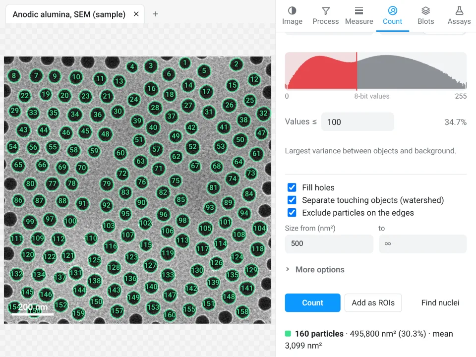
- Pore size and porosity (AAO, porous films): count the dark pores with a circularity range for their areas and equivalent diameters; the share of the image on the pore side of the threshold, shown next to the threshold value, is the porosity (the Summary row's %Area counts only the pores that are not cut by the frame).
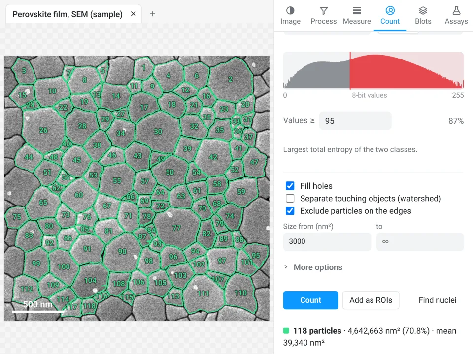
- Grain size of thin films: threshold the grains so that their darker boundaries stay closed (MaxEntropy often suits secondary-electron images; the Pixel classifier helps when the contrast is uneven), add watershed only where a boundary is open, then count them for the grain areas and equivalent diameters.
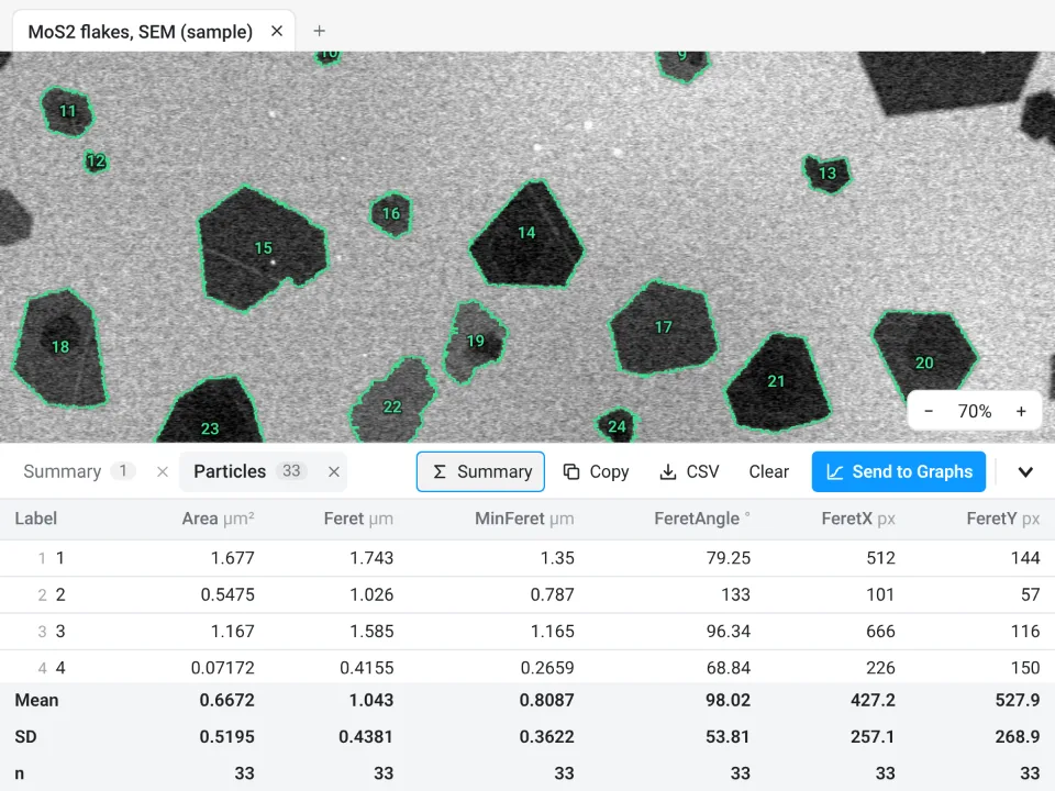
- Lateral size of 2D flakes: count the flakes, or train the classifier on flake and substrate, and read the Feret diameters.
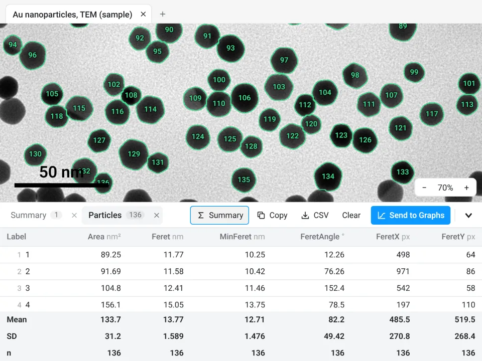
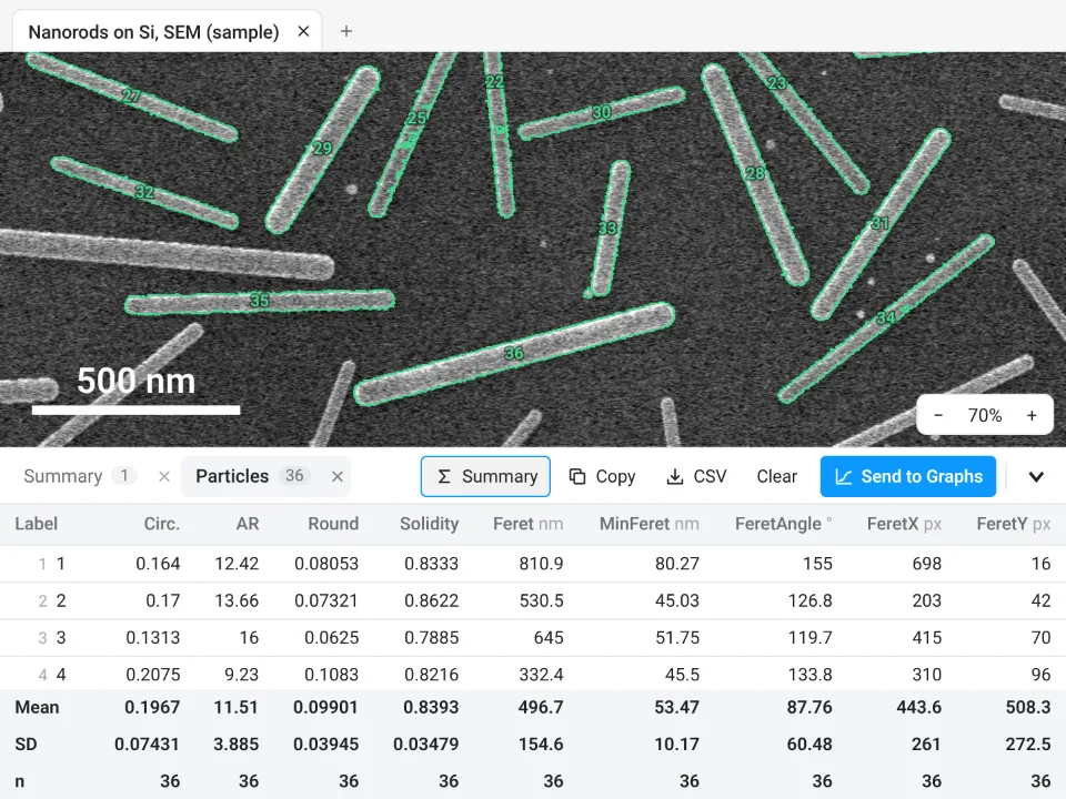
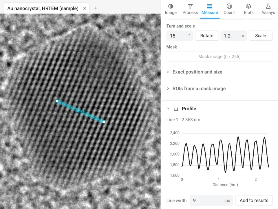
The rest of this guide goes through every tab, tool and setting.
The app is organised in six tabs on the right (Image, Process, Measure, Count, Blots, Assays), a tool rail on the left, the image in the middle and a results drawer underneath. Sections fold: click a title to fold it, Alt-click to show that section alone.
Where to find the commands you know
| If you are used to | In LabCanvas Image Analysis |
|---|---|
| ROI Manager, Measure, Set Measurements | Measure tab: the ROI list, Measure, Measure all ROIs, Set measurements |
| Analyze Particles | Count tab › Count particles (fill holes, watershed, size, circularity, exclude on edges) |
| Threshold, Make Binary, Fill Holes, Watershed, Skeletonize, Distance Map, Ultimate Points | Process › Binary; Count › Count particles |
| Subtract Background (rolling ball, sliding paraboloid) | Process › Background and filters › Background |
| Gaussian Blur, Median, Mean, Minimum, Maximum, Unsharp Mask | Process › Background and filters › Filter |
| Enhance Local Contrast (CLAHE), Remove Outliers, Despeckle, FFT Bandpass | Process › Enhance |
| Image Calculator, Ratio images | Process › Calculator |
| Colour Deconvolution, Colour Threshold | Process › Colour deconvolution, Colour threshold |
| Drift and channel registration | Process › Align |
| Brightness/Contrast, Lookup Tables, Channels Tool, Calibration Bar | Image › Display |
| Set Scale, Scale Bar | Image › Scale |
| Z Project, Orthogonal Views, Reslice, Make Substack, Reduce, Animation | Image › Stack and image |
| Plot Profile, Plot Z-axis Profile | Measure › Profile |
| Colocalisation (Pearson, Manders, Costes) | Measure › Colocalisation |
| Enlarge, Make Band, Combine/AND/XOR, Convex Hull, Fit Ellipse, Specify | Measure › ROI tools |
| Find Maxima | Count › Spots |
| Cell Counter | Count › Cell counter |
| Trainable segmentation | Count › Pixel classifier |
| Batch processing | Count › Batch, and Run on many images in every assay |
| Gel lanes and peaks | Blots tab |
| Tracking, kymographs, skeleton analysis, Sholl, angiogenesis networks | Assays tab |
Opening images
Click Open an image, press Ctrl O, drop files on the window or paste. Four samples are on the start screen (a western blot, nuclei, two channels for colocalisation and a 15-slice Z-stack) and every assay has its own.
- TIFF and BigTIFF: strips or tiles, uncompressed, LZW, Deflate or PackBits; 8- and 16-bit kept as they are, other depths (signed, 32-bit, float) read as 32-bit float. Every page is read; pages of another size (thumbnails, pyramid levels) are left out with a note.
- Hyperstacks and OME-TIFF: channels, slices, frames, pixel size, slice spacing, frame interval and channel names come from the file's description. Otherwise the resolution tags are used, but only in centimetres (an inch DPI is a print size, not a pixel size).
- PNG, JPEG, WebP, GIF, BMP: read at 8 bits; a grey picture becomes one channel, a colour picture three. JPEG gets a warning that compression changed the pixel values.
- ROIs: .roi files and RoiSet.zip (rectangles, ovals, polygons, freehand, traced, straight, segmented and freehand lines, angles, points, composite shapes, with names, colours and positions) go to the image shown.
- Projects: a .lcanalysis file holds every image (as TIFF, raw values and scale), its ROIs and all results tables. The session also saves itself in the browser and comes back after a reload.
- Files in a microscope maker's own format (.czi, .nd2, .lif, .lsm, .oib, .vsi, .ims and others) are not read in the browser: export them as TIFF from the acquisition software (OME-TIFF keeps the scale and the channels).
The File menu also has Save image as TIFF (raw values, hyperstack layout and scale), Download PNG (as shown, with the scale bar), Add to a figure and Add channels to a figure.
Drawing and editing ROIs
The tool rail: Rectangle (R), Oval (O), Polygon (G), Freehand (F), Line (L), Points (P), Wand (W) and Pan (H, or hold Space). Shift draws a square or circle. A polygon closes on its first point, a double-click or Enter. The wand traces the object under the click: the red object of the threshold preview when it is on, otherwise the connected pixels within the tolerance set in Count. Click selects an ROI, Shift-click adds, drag moves, handles resize, Delete removes. The readout under the cursor shows x, y, the calibrated position and the value of every channel. Undo keeps 40 steps (Ctrl Z, Ctrl Shift Z).
The Image tab
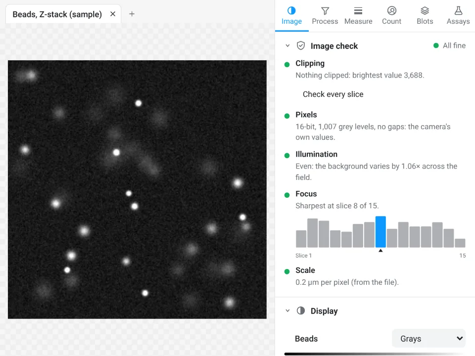
Image check
Is the image fit to measure? The check runs on opening, folds itself away when all is fine and opens when something needs attention:
- Clipping: the share of pixels at the top value or at 0, per channel and inside the selected ROIs; Show where marks them in red and blue; Check every slice goes through a stack.
- Pixels: the bit depth and the number of grey levels; flags a picture taken from a figure, a JPEG, or gaps in the histogram left by earlier processing.
- Illumination: how much the background varies across the field (a warning above 1.3×), with a link to correct it.
- Focus: a sharpness score, and for stacks a bar per slice with the sharpest one marked and Go to the sharpest slice.
- Scale, and with several images open, Open images: a table of their type, pixel size and size that flags images that cannot be compared fairly.
Display
Display changes only how the image looks. Composite, One channel or Gray; for each channel an eye to hide it, a lookup table (Grays, Red, Green, Blue, Cyan, Magenta, Yellow, Fire, Ice, Viridis, Inferno, Spectrum, Inverted grays), a histogram with the display ramp, minimum and maximum sliders and fields, Auto (saturates 0.35% of the pixels at each end) and Full. Sliders move through Channel, Slice and Frame. Colour scale bar draws a calibration bar for false-colour images, in a corner you choose, with white or black text and a title such as "Ratio 405/488". The footer reminds you which raw bit depth is measured.
Scale
Draw a line along a scale bar or a micrometer, type the Known distance and the Unit (µm, nm, mm, cm, m, Å) and click Set scale; or type the pixel size directly. Scale bar adds a bar with its Length, Position, Thickness, Text size, white or black, and a Label.
Stack and image
- Player: Play and Pause through frames or slices at a frame rate you set, with Loop.
- Orthogonal views: XZ and YZ strips through a point you pick; XZ as image, YZ as image and Reslice along a selected line.
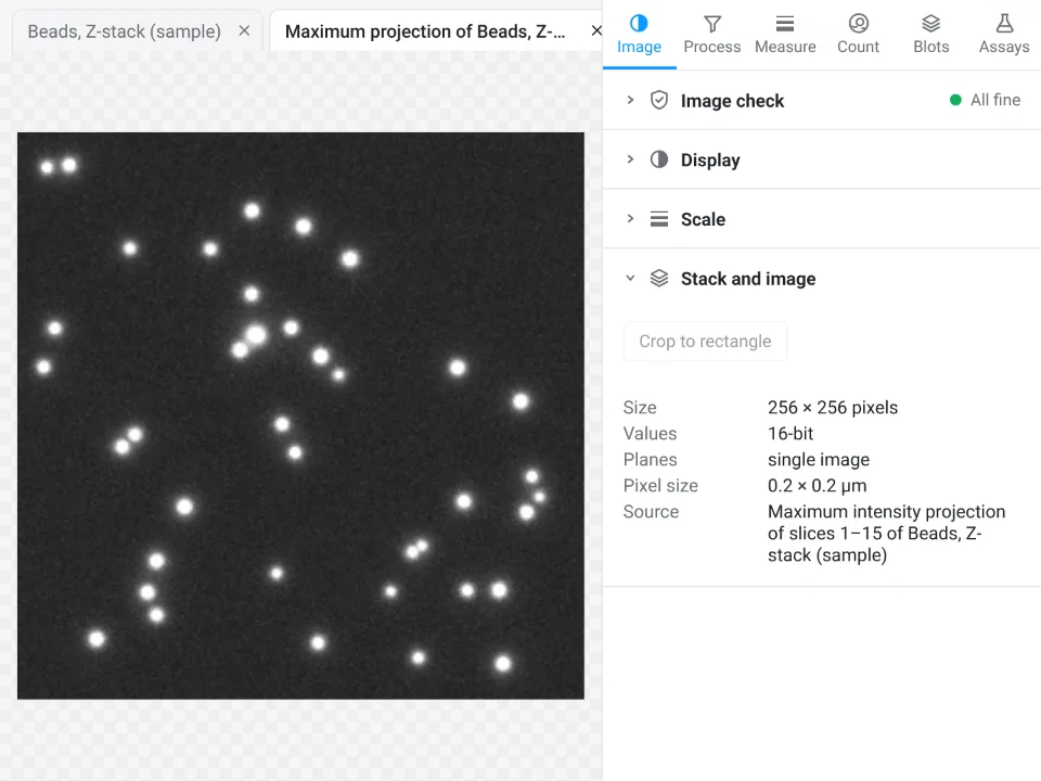
- Z projection: Maximum, Average, Sum, Standard deviation, Minimum or Median, over the slices you choose, as a new image.
- Substack and reduce: a substack of the slices or frames you choose, every n-th, and Reduce to keep every n-th plane.
- Channel as image, Crop to rectangle, and an info list (size, values, planes, pixel size, slice spacing, frame interval, source).
The Process tab
Every Process step can apply to all channels and planes or only to the ones you choose, optionally As a new image and as a 32-bit result, with progress and Cancel on long stacks. Each step is undoable.
Background and filters
- Background: Rolling ball radius (at least the radius of the largest object that is not background), Light background, Sliding paraboloid, Smooth first, a Preview of the background and the result, then Subtract background or Background as image.
- Filter: Gaussian blur (sigma), Median, Mean, Minimum, Maximum (radius) and Unsharp mask (sigma and weight).
- Bit depth: convert to 8-, 16- or 32-bit, scaled to the display range or not.
Enhance
For seeing and segmenting, not for measuring intensities (the panel says so). Local contrast (CLAHE) with tile size, clip limit and bins; Denoise (non-local means) with strength, patch and search sizes, the noise estimated for you; Remove outliers, bright or dark, with radius, threshold and a preview of the pixels that would change; Despeckle; and FFT bandpass (remove structures larger and smaller than sizes you give, optionally horizontal or vertical stripes).
Binary
On a grey image: pick a Threshold method (Default (IsoData), Otsu, Huang, Intermodes, IsoData, Li, MaxEntropy, Mean, MinError, Minimum, Moments, Percentile, RenyiEntropy, Shanbhag, Triangle, Yen, or a value), bright or dark objects, preview it in red, and Make binary. On a mask: Erode, Dilate, Open, Close (by steps or by a distance in calibrated units), Fill holes, Outline, Skeleton, Watershed, Distance map and Ultimate points (with their radius in a table).
Calculator
- Two images: Subtract, Add, Multiply, Divide, Average, Difference, Minimum, Maximum, AND, OR and XOR between any two channels of open images of the same size, as a 32-bit result if you like; a single-plane image is applied to every plane of a stack.
- Ratio: A ÷ B with background values and a threshold estimated for you (or taken from an ROI); dim pixels become NaN, and the 32-bit ratio image opens with the Fire table and a colour scale bar. The median and mean ratio per plane go to a table.
- One image: add, subtract, multiply or divide by a value, Log, Exp, Square root, Square, Reciprocal, Invert, or set the background to NaN.
Align
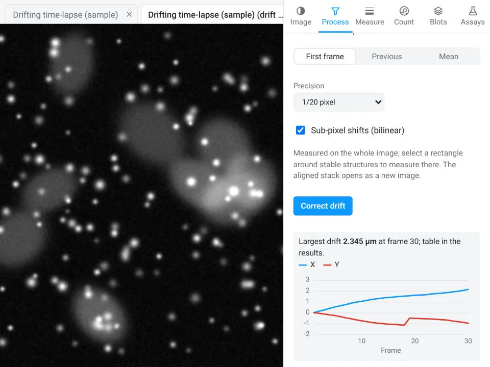
Drift: line each frame (or slice) up with the first, the previous or the mean, measured on a channel you choose, to whole, 1/10, 1/20 or 1/100 pixel, with sub-pixel shifts, on the whole image or inside a rectangle around stable structures. The aligned stack opens as a new image and the drift of every frame goes to a table and a chart. Channels measures and corrects the shift between two channels (chromatic shift).
Colour deconvolution and colour threshold
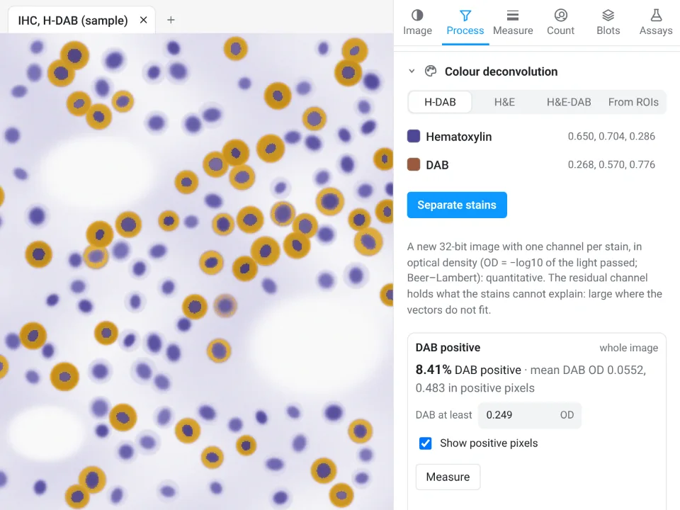
For colour pictures of stained sections. Colour deconvolution separates H-DAB, H&E or H&E-DAB, or stains you measure yourself on ROIs, into a 32-bit optical-density image with one channel per stain (and a residual channel). When one stain is DAB, a DAB positive block gives the DAB-positive area and the mean DAB optical density, with a threshold set automatically (or by you), per ROI or for the whole image. Colour threshold selects pixels by Hue, saturation, brightness or **L\*a\*b\*** around colours you pick (Shift-click adds a colour) with a tolerance, then measures the colour area, makes ROIs or a mask.
The Measure tab
Measure and Set measurements
The ROI list shows every ROI with its kind, name and size: click to select, Shift or Ctrl to add, double-click or F2 to rename, arrows to move. Import… and Export RoiSet.zip move ROI sets in and out. Measure measures the selected ROIs (or the whole image), Measure all ROIs measures every one, on This channel or All channels, and on this plane or Every slice or Every frame. Set measurements chooses the columns:
- Area, Mean, Min and max and Integrated density (on by default);
- Standard deviation, Median, Centroid, Centre of mass, Perimeter;
- Shape descriptors (circularity, aspect ratio, roundness, solidity), Fit ellipse (major, minor, angle) and Feret's diameter (Feret, MinFeret, angle and start point).
The table columns are the familiar ones: Area, Mean, StdDev, Min, Max, Median, IntDen, RawIntDen, X, Y, XM, YM, Perim., Circ., AR, Round, Solidity, Major, Minor, Angle, Feret, MinFeret, FeretAngle, FeretX and FeretY. Lines give their length and angle and the values along them; points give their count.
ROI tools
- Combine, Intersect, XOR and Subtract (the first minus the others).
- Enlarge, Shrink and Band (a ring; rings of neighbours are split halfway), by a distance in pixels or calibrated units.
- Hull, Ellipse, Circle (fitted) and Split (a composite ROI into its pieces); Rotate and Scale.
- Mask image from the ROIs; ROIs from a mask image (objects or label values); and an Exact position and size dialog for rectangles and ovals.
Profile
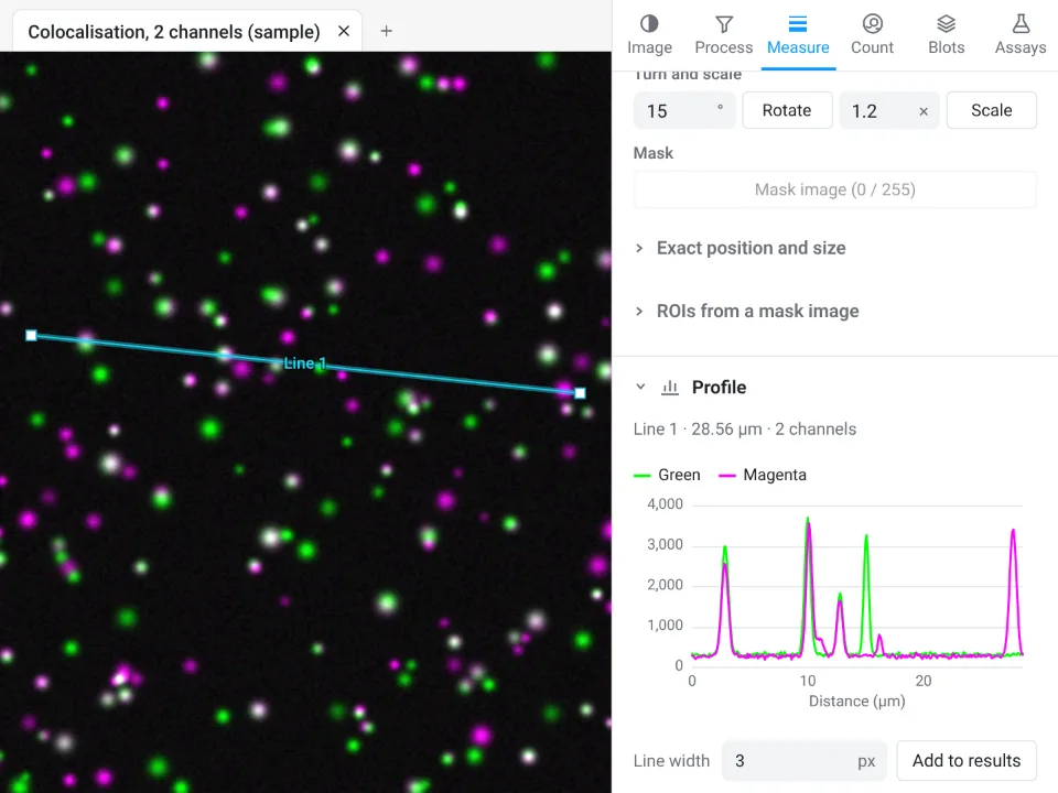
With a line selected, a live plot of the values along it, one curve per channel, with a Line width for a wider average; hovering the plot marks the point on the image. With no line on a stack, the mean of the selected area through slices or through time (a Z-axis or time profile). Add to results puts the numbers in a table.
Colocalisation
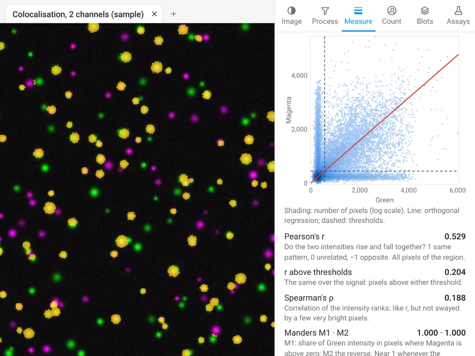
Choose two channels, a region (the selected ROI or the whole image), all slices of a Z-stack or one, and the thresholds: Costes (auto), values you set, or none. Calculate draws the 2D histogram with its regression line and gives Pearson's r, r above the thresholds, Spearman's ρ, Manders M1 and M2, thresholded tM1 and tM2, the overlap coefficient and Li's ICQ; Show colocalised marks the pixels above both thresholds in yellow. Each run adds a row to the Colocalisation table.
The Count tab
Count particles
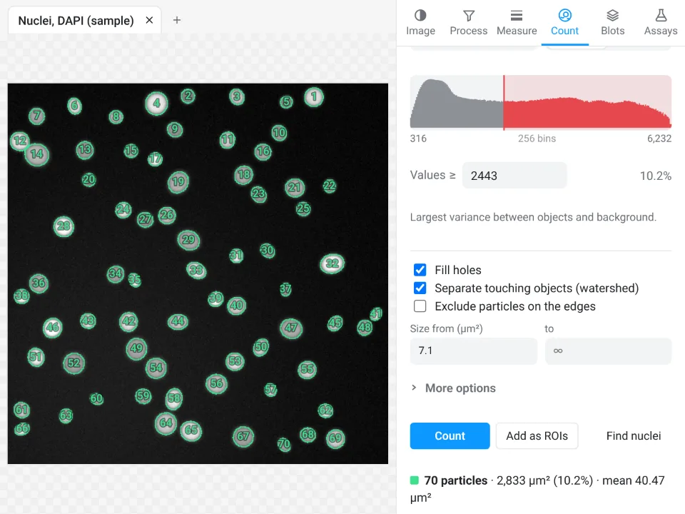
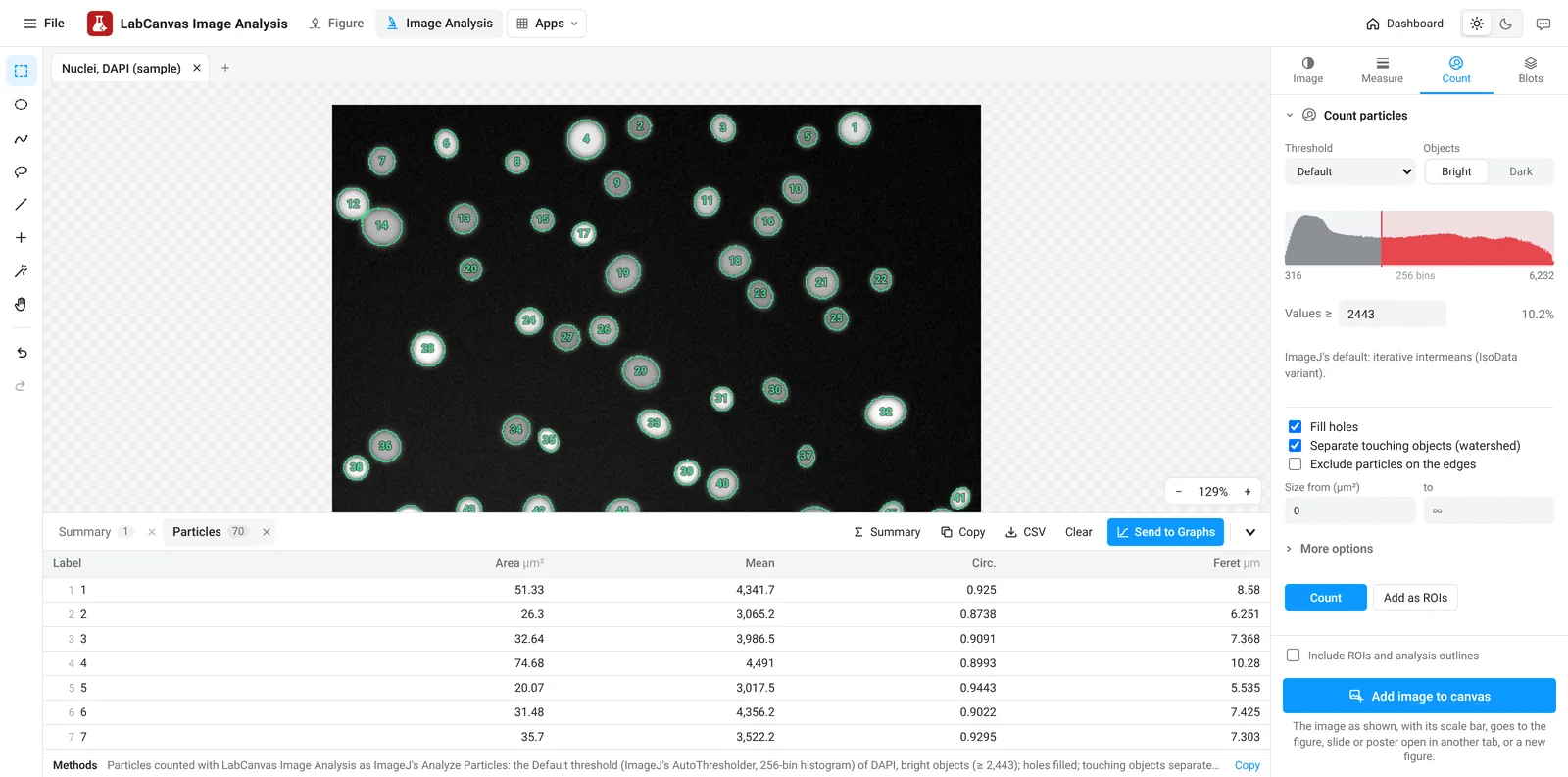
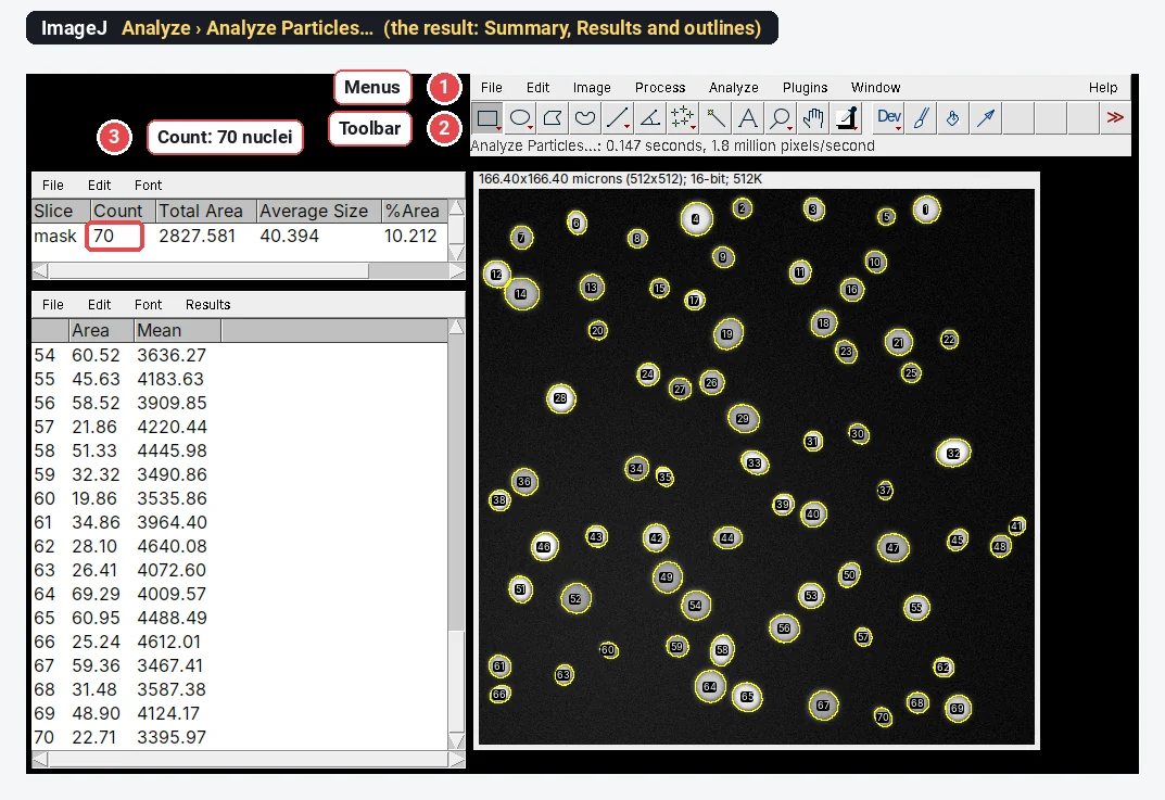
The everyday Analyze Particles. Objects come from a Threshold (any of the sixteen methods or a manual cut set by dragging on the histogram, bright or dark objects, on a channel you choose, previewed in red) or from the Classifier below. Options: Fill holes, Separate touching objects (watershed), Exclude particles on the edges, Only inside the selection, a size range, a circularity range, sizes in pixels or calibrated units, and which image to Measure (the thresholded channel, another channel or another open image of the same size). Count outlines and numbers every particle and fills a Particles table and a Summary row (Count, Total Area, Average Size, %Area, Mean); Add as ROIs sends them to the ROI list; Find nuclei does Otsu, fill holes, watershed and a sensible minimum size in one click.
Pixel classifier
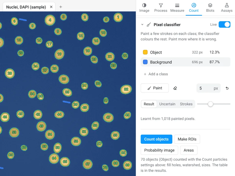
When a threshold cannot separate what you want, paint a few strokes on each class (Object and Background to start, up to six classes) and a random forest of 100 trees colours the rest, live; paint more where it is wrong. The brush has a size and an eraser (or hold Alt); the view shows the Result, the Uncertain pixels or your Strokes. Count objects counts with the Count particles settings, Make ROIs makes ROIs, Probability image gives one 32-bit channel per class and Areas measures the area of each class. Detail (fine, medium, coarse) sets the scale of the features it looks at; a classifier can be saved and loaded.
Spots
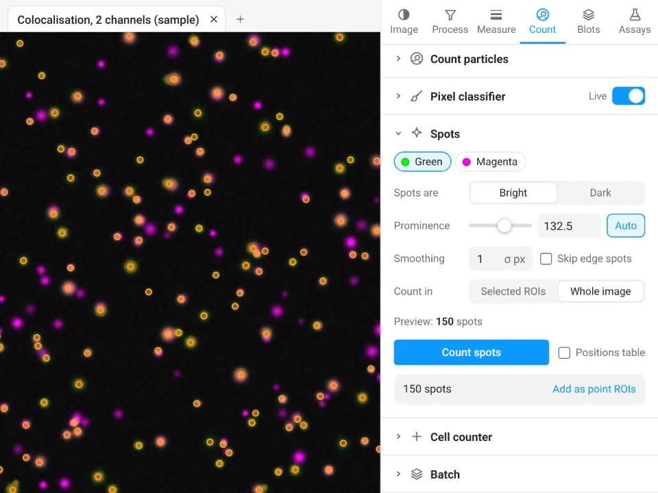
Find Maxima for puncta, foci and beads: bright or dark spots, a Prominence set automatically from the image's noise (or by you), Smoothing, Skip edge spots, counted in the selected ROIs or over the whole image, with a live preview of every spot. The table gives the count, area and density per ROI, and optionally every spot's position and value; Add as point ROIs keeps them.
Cell counter and Batch
The Cell counter counts by clicking, in up to 20 named categories (keys 1 to 9 switch between them; a click on a marker removes it), and gives the count, total and percentage per category, with optional marker positions and their values. Batch runs the Count particles settings on every open image or on files you choose, opened one at a time: one Summary row per image, and every particle if you want them.
The Blots tab
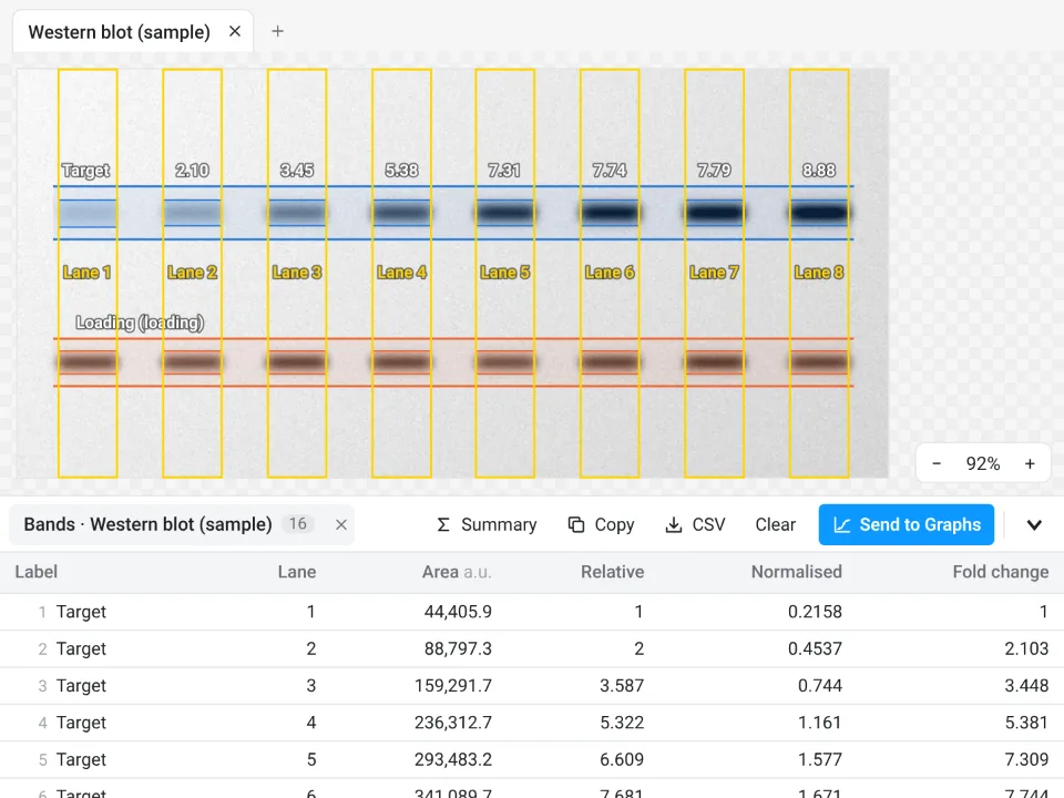
Western blot and gel densitometry in three steps. Band look (dark or light bands) is detected from the image.
- Lanes: vertical or horizontal; Find lanes, Add lane or Use selected rectangles, the same width for every lane. Choose a Molecular-weight ladder lane and type its sizes (for example 250, 150, 100, 75, 50, 37, 25, 20, 15, 10 kDa), with a straight or curved fit, to read every band's size.
- Bands: Find bands proposes the band rows across lanes; drag their windows on the image or on the lane plot, name them and mark the loading control. Align lanes corrects smiling or shifted lanes before bands are matched.
- Quantify: a Background under each band (Straight line, Rolling or None), Normalise to a loading-control band or a Total protein stain image (Ponceau S, stain-free, with an offset if it is not aligned), and a Reference lane. The table gives each band's area, its value relative to the reference lane, the normalised value and the fold change, the lane's total protein and the band's molecular weight; it updates as you change anything. Lane profile shows each lane's plot with its band windows.
The Assays tab
Guided measurements for common experiments. Each opens as numbered steps with settings that work in one click, shows its result on the image as you change a setting, offers Try it on a sample, and ends in tables you can send to Graphs. Save as workflow keeps an assay's settings under a name, listed at the top of the tab; a workflow runs on every open image or on files (Run on N open, Files…), and the results collect in one table, a row per image or per cell.
Nuclear vs cytoplasmic signal
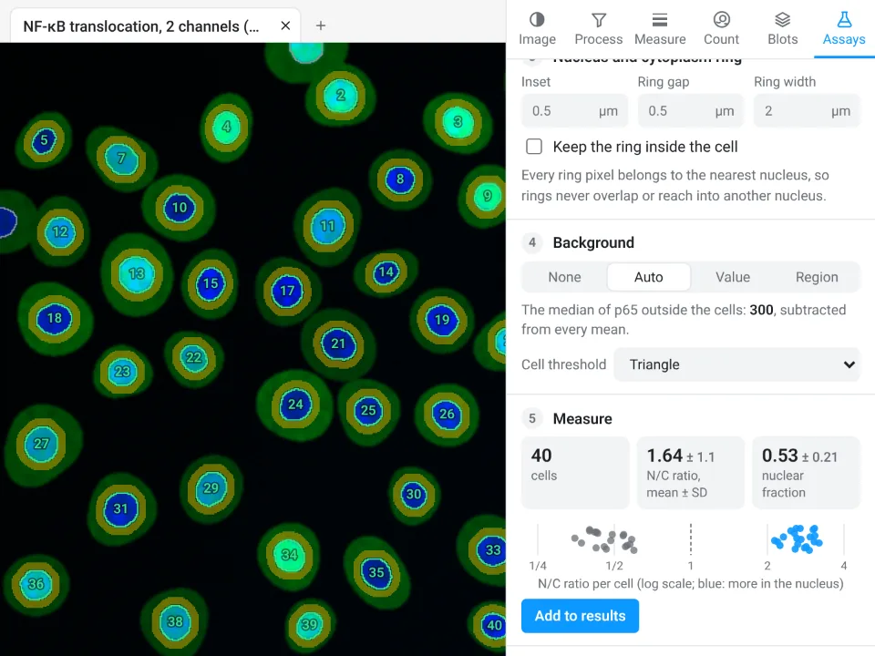
For NF-κB, YAP or TFEB translocation (two channels: nuclei and signal). Nuclei are found with a threshold (Otsu by default), blur, a smallest size, fill holes, split touching nuclei and leave out nuclei on the edge; a cytoplasm ring is drawn around each with an Inset, Ring gap and Ring width (rings never overlap a neighbour, and can be kept inside the cell). Background: none, automatic, a value or a region. Per cell: nucleus and ring area, mean and integrated density, the N/C ratio and the nuclear fraction, plus a summary.
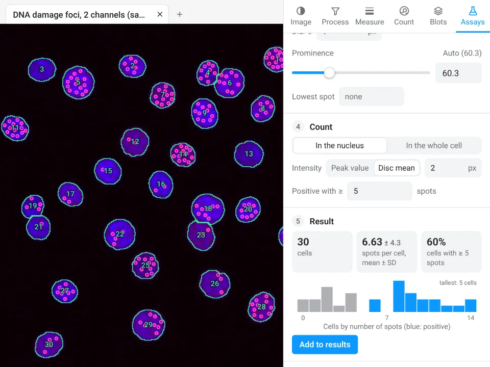
Spots per cell
For γH2AX, 53BP1 or LC3 foci. The same nuclei step, then spots with optional background removal, blur and a prominence set from the noise; counted in the nucleus or in the whole cell (a distance around the nucleus), with the peak value or a disc mean as intensity, and a number of spots that makes a cell positive. Per cell: spots, mean and total spot intensity, spots per area; and the share of positive cells.
Colony counting
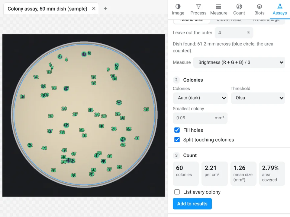
In a Round dish (found automatically, leaving out a rim), in Drawn wells, or over the whole image; dark-on-light or light-on-dark colonies, a threshold, a smallest colony, fill holes and split touching colonies. Gives the count, colonies per cm² on a calibrated image, mean size and diameter and the area covered, and if you like every colony's size.
Wound healing (scratch)
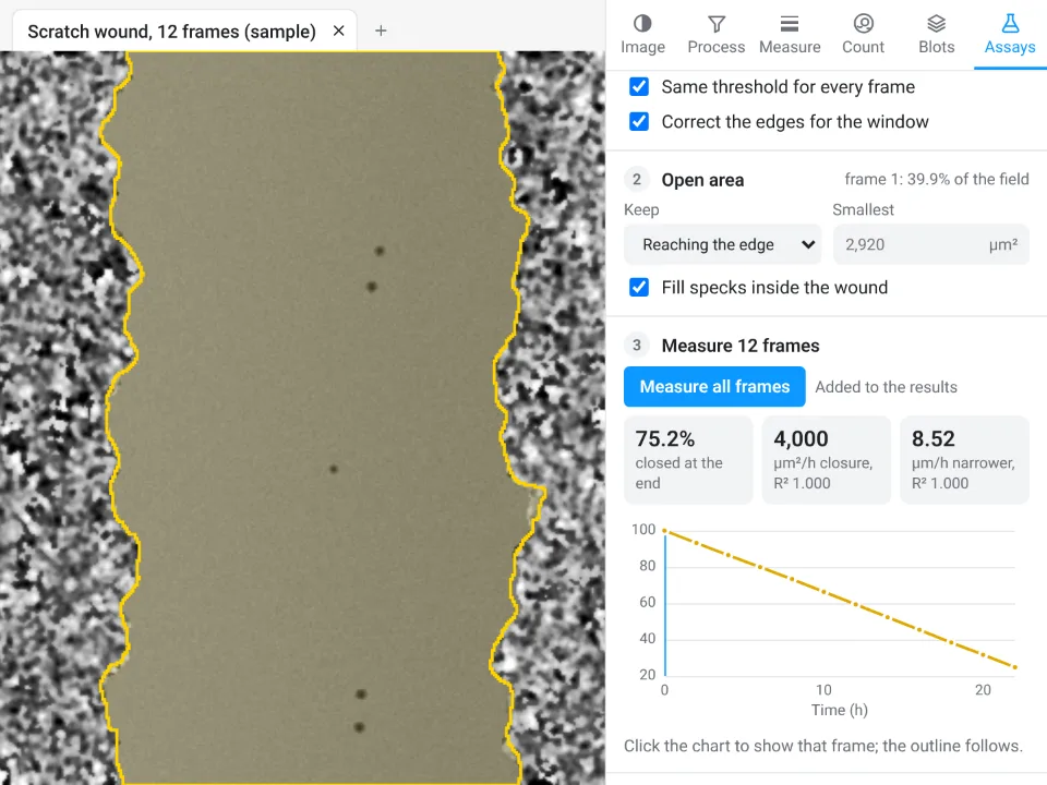
The open area of a scratch from the image's texture (a window radius and a threshold, the same for every frame), keeping the region that reaches the edge, the largest or all, and filling specks inside it. On a time-lapse, Measure all frames gives the open area, % of initial area, % closure and mean width over time, and the closure rates (area and width per hour, with their R²); one image gives its open area and width.
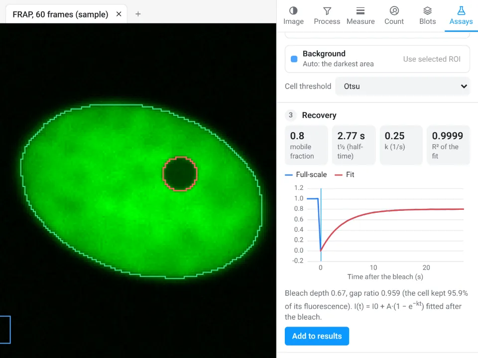
FRAP recovery
The bleach frame is found automatically; the bleached spot, the reference (whole cell) and the background are found too, or taken from ROIs you draw. The recovery is double normalised, scaled to full scale and fitted with
Calcium traces (ΔF/F₀)
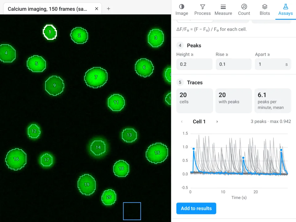
Cells found on a standard-deviation, maximum or mean projection (or your own ROIs), background removed, a baseline F₀ from a low percentile or the first frames, and peaks above a height, a rise and a minimum spacing. Per cell: area, F₀, number of peaks, maximum ΔF/F₀, first peak, frequency and area under the curve, plus every trace in one table and an interactive chart.
Track particles and cells
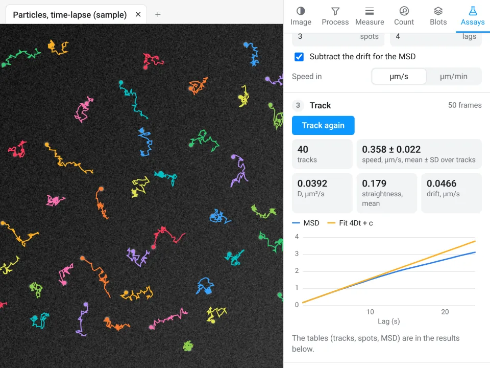
Detect spots or objects in every frame, then link them into tracks with a largest move, missed frames allowed and a shortest track. Per track: duration, path length, net displacement, mean and maximum speed and straightness; the mean squared displacement (with the drift subtracted if you like) is fitted for the diffusion coefficient D. Tracks are drawn in colour on the image.
Kymograph
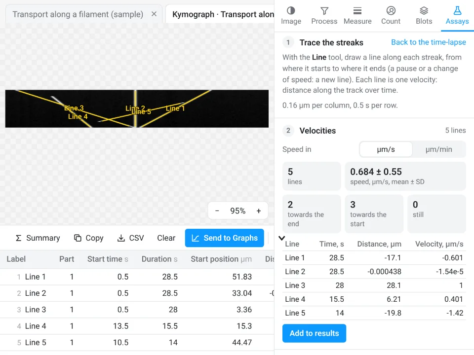
Draw or trace a line along a filament or axon (or let Find the track find the brightest one), set its width and Make kymograph: distance across, one row per frame. Then draw lines along the streaks: each gives its velocity, and the summary splits them into moving towards the end, towards the start and still.
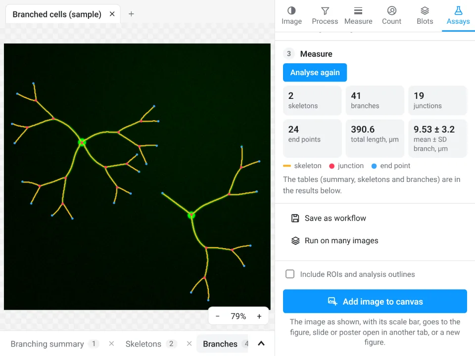
Branching and skeleton
For neurites, vessels, hyphae or filaments: find the structures with a threshold (Li by default), smoothing, smallest object and holes to fill, prune short spurs, and Analyse. Gives skeletons, branches, junctions, end points, triple and quadruple points, total, mean and maximum branch length, and every branch with its length, straight-line distance and tortuosity.
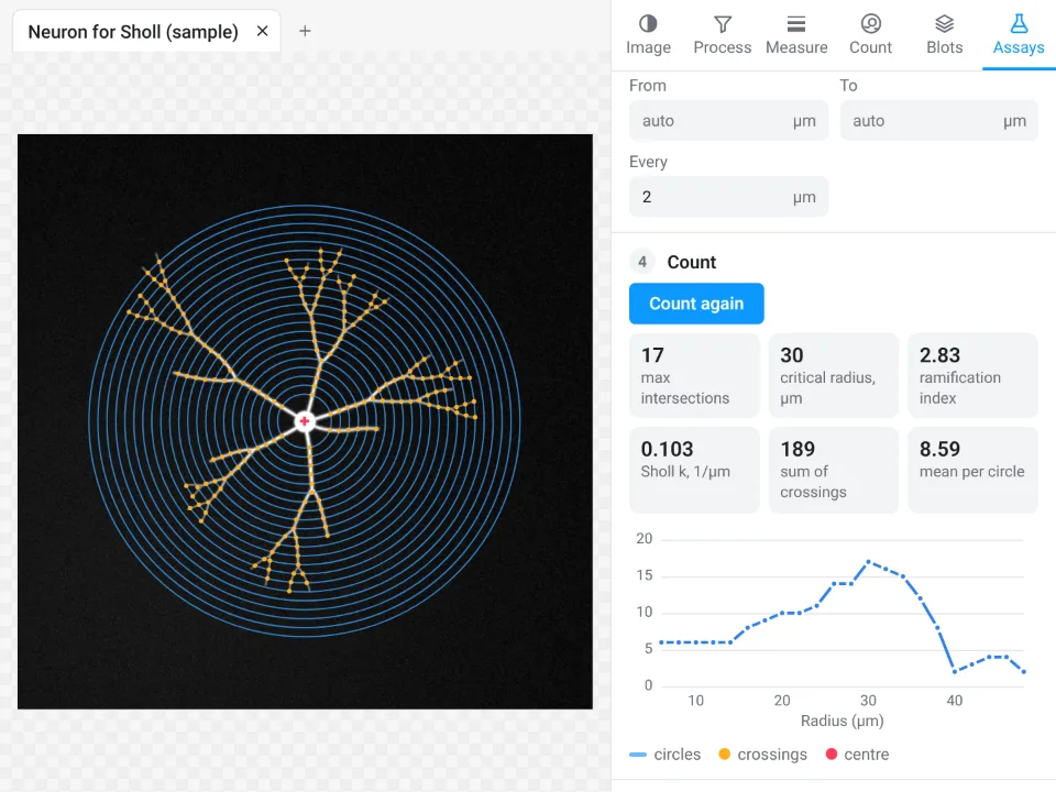
Sholl analysis
The cell is found as for branching, counted on the cell or on its skeleton, around the cell body (found automatically) or a centre you click, on circles from a start to an end radius in steps you set. Gives the Sholl profile, the maximum number of crossings and its critical radius, the sum and mean, primary branches, the ramification index and the Sholl regression coefficient k with its R².
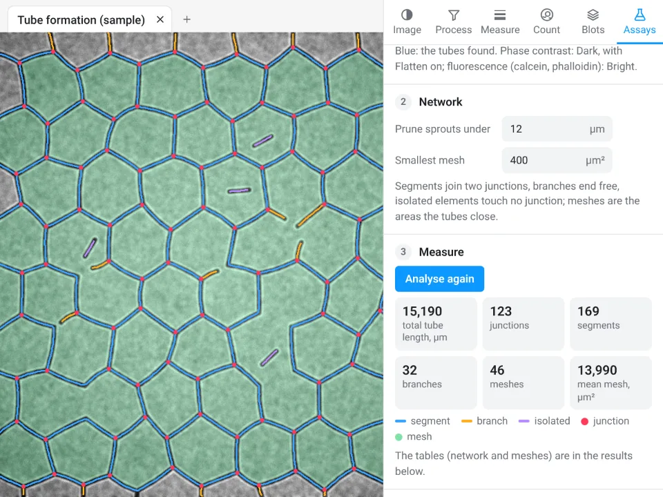
Tube formation
Endothelial networks on matrix, in phase contrast or fluorescence: the tubes are found (with background flattening), short sprouts pruned and meshes smaller than a size left out. Gives total tube length, segments, branches, isolated elements, junctions, meshes and their total and mean area.
Results, and where they go
Every table sits in the results drawer under the image, one tab per table, with units in the column headers. Click a row to select its ROI and image. Above each table:
- Summary adds Mean, SD and n rows; Copy puts the table on the clipboard for a spreadsheet; CSV saves it; Clear empties it.
- Send to Graphs makes a Graphs data table with a graph from the column you pick: By image (one data set per image, for example control and treated), All rows, or XY for profiles, time series and other tables with a position column. Sending the same table again updates the same graph.
- Methods: each table carries a sentence describing how it was measured (on which values, with which definitions and pixel size), ready to copy into the methods section.
Images go to figures too: Add image to canvas places the image as shown, with its scale bar (and its ROIs and outlines if you tick that), in the figure, slide or poster open in another tab; Each channel and the merge sends every channel and the merge as separate pictures side by side for a panel layout, single channels in grey if you like.
Keyboard shortcuts
| Keys | Action |
|---|---|
| R, O, G, F, L, P, W, H | Rectangle, Oval, Polygon, Freehand, Line, Points, Wand, Pan |
| Space (hold) | Pan |
| Ctrl Z, Ctrl Shift Z | Undo, redo |
| Ctrl O, Ctrl S | Open, save the project |
| +, −, 0, 1 | Zoom in, zoom out, fit to window, 100% |
| Delete | Remove the selected ROIs |
| F2 or Enter | Rename the selected ROI or category |
| 1 to 9 | Switch categories in the cell counter |
| Esc | Stop a tool, cancel a polygon, deselect |
Good practice
- Measure the original file from the instrument, not a picture exported for a figure: JPEG compression and adjustments change pixel values. The image check flags both.
- Keep acquisition settings the same for images you compare, avoid clipped pixels, and measure them with the same settings: saved workflows and Batch make that easy.
- Enhance and denoise to see and to segment; measure intensities on the original image.
- For blots, stay within the linear range of the detection and normalise to a loading control or total protein.
Every measurement here is checked against independent software and against images with known answers, in more than 4,000 automated tests: see how Image Analysis is validated. Ready to try it? Open Image Analysis and click a sample.
Frequently asked questions
Will it feel familiar if I already measure images on the desktop?
Yes. The tools carry the names you know: an ROI list with Measure and Set measurements, Analyze Particles with fill holes, watershed, size and circularity, rolling-ball background subtraction, the usual automatic threshold methods (Default IsoData, Otsu, Li, Triangle, Huang, MaxEntropy, Yen and the rest), Z Project, Orthogonal Views, Reslice, Find Maxima, Cell Counter, Plot Profile, gel lanes, colour deconvolution, a calibration bar and a scale bar. ROI sets (.roi, RoiSet.zip) and hyperstack TIFFs open and save in the usual formats.
Do the display settings change my measurements?
No. Brightness, contrast and lookup tables change only how the image is shown. Every measurement, threshold, assay and blot reads the raw 8-, 16- or 32-bit values, and the image check warns when the data are clipped, compressed or came from a figure rather than the instrument.
Which threshold methods are there?
Default (IsoData), Otsu, Huang, Intermodes, IsoData, Li, MaxEntropy, Mean, MinError, Minimum, Moments, Percentile, RenyiEntropy, Shanbhag, Triangle and Yen, plus a value you set by hand or by dragging on the histogram.
Can I run the same measurement on a whole folder of images?
Yes. Counting has a Batch section that runs the Count particles settings on every open image or on files you choose. Every guided assay except the kymograph can be saved as a workflow and run on many images; the files are opened one at a time and the results collect in one table, one row per image or per cell.
Which files open?
TIFF and BigTIFF (stacks, hyperstacks, 8-, 16- and 32-bit, OME-TIFF), PNG, JPEG, WebP, GIF and BMP, ROI files (.roi, RoiSet.zip) and LabCanvas projects (.lcanalysis). Files in a microscope maker's own format (.czi, .nd2, .lif and others) need to be exported as TIFF first; OME-TIFF keeps the scale and channels.
Try it in LabCanvas
Every app is free to start in your browser. Create an account and begin.
Start Image Analysis free in your browserKeep reading
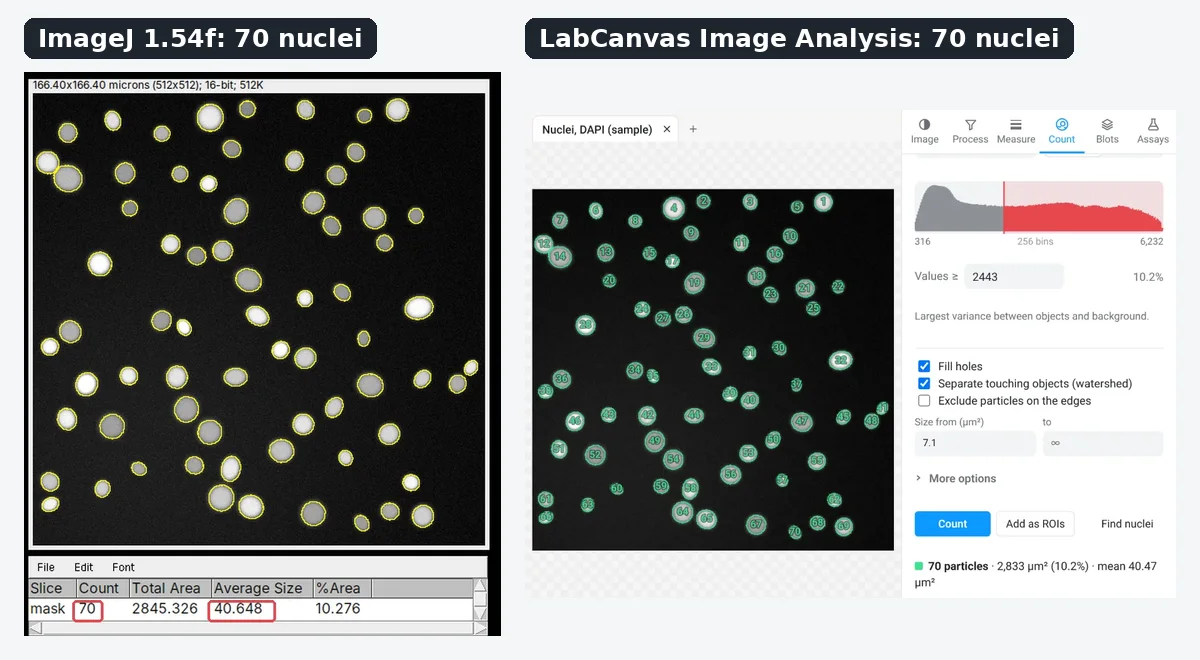
ImageJ vs LabCanvas Image Analysis: an honest comparison
ImageJ/Fiji or LabCanvas Image Analysis? Six everyday jobs done in both, six newer ones (macros, vendor files, 3D, StarDist, big images) and which to use.
LabCanvas Image Analysis: measure microscopy images, western blots and gels in your browser
How to measure images in LabCanvas Image Analysis: guided assays (nuclear translocation, spots per cell, wound healing, FRAP, calcium, tracking, branching), western blots with a ladder and total-protein normalisation, cell counting with a trainable classifier, ROIs with ImageJ definitions, on the raw pixel values, with results sent to Graphs.
How to use ImageJ: a beginner's tutorial for the 10 everyday jobs (2026)
How to use ImageJ and Fiji: get started, open an image, then 10 everyday jobs (scale, measure, threshold, count, background, blots) with exact menu paths.