ImageJ vs LabCanvas Image Analysis: an honest comparison
ImageJ/Fiji or LabCanvas Image Analysis? Six everyday jobs done in both, six newer ones (macros, vendor files, 3D, StarDist, big images) and which to use.
Contents
Choose ImageJ (in practice, Fiji) if your method depends on a plugin, on a macro with loops and variables, on time-lapse tracking with TrackMate, or on a file format LabCanvas cannot read, or if the software must run offline with its source open: its plugin ecosystem is far larger than anything else, and it is free with no account. Choose LabCanvas Image Analysis for the everyday measurements (counts, sizes, blots, intensities, colocalisation, scale bars) when you want them in a browser with nothing to install, guided step by step, checked before you measure and sent straight to statistics and figures. Since November 2026 it also records analyses as recipes you can run on a folder and export as ImageJ macros, opens DICOM and the main microscope formats, segments and measures 3D objects, finds nuclei with StarDist, deconvolves, stitches tiles and opens whole-slide images tile by tile, each with limits listed below.
We make LabCanvas, so we have tried hard to be fair. Jobs 1 to 6 below were done in both programs on the same synthetic sample image, with real screenshots of each. Jobs 7 to 12 cover the newer LabCanvas features: we show LabCanvas screenshots and describe the Fiji route in words, because we did not repeat those jobs in Fiji. ImageJ and Fiji are independent open-source projects; LabCanvas is not affiliated with them.
How we compared: ImageJ 1.54f (the commands are the same in Fiji) and LabCanvas Image Analysis in Chromium, on synthetic samples with known answers: 70 nuclei at 0.325 µm per pixel, gold nanoparticles at 0.25 nm per pixel, an 8-lane western blot with known band amounts, a stage micrometer, and a two-channel colocalisation image. The ImageJ screenshots come from our step-by-step ImageJ guides, which give every menu path. Jobs 7 to 12 show LabCanvas only, on its test images; no ImageJ numbers are given for them.
Who each tool is for
ImageJ is the general-purpose image analysis program of the life sciences, developed at the US National Institutes of Health since 1997 and descended from NIH Image (Schneider et al. 2012). Fiji is ImageJ with hundreds of plugins and an updater, aimed at biological image analysis (Schindelin et al. 2012). They are for:
- anyone who needs a measurement no other program has: there is a plugin or macro for almost everything;
- people who analyse the same way many times and can write, or record, a macro, including loops, conditions and calls to plugins;
- time-lapse tracking (TrackMate), 3D analysis with the many 3D plugins, and deep-learning models beyond fluorescent nuclei;
- labs with vendor files in any of about 150 formats, read through Bio-Formats (Linkert et al. 2010);
- work that must run offline, on open-source software, with no account.
LabCanvas Image Analysis is a browser app that measures microscope images, western blots and gels on their raw values, with ImageJ's measurement names. It is for:
- students and scientists who need a standard measurement done right without learning which commands to run in which order;
- computers where you cannot install software, and tablets;
- assays that need a plugin or a macro in ImageJ: nuclear translocation, spots per cell, AI nucleus segmentation, colonies, wound healing, FRAP, calcium imaging, tracking, kymographs, branching, Sholl analysis and tube formation, each a guided panel with a sample image;
- the common heavier jobs without setting anything up: recipes run on a folder, microscope and DICOM files, 3D objects, StarDist, deconvolution, stitching and whole-slide viewing;
- going from the numbers to statistics, figures and a methods sentence in one place.
The comparison table
| ImageJ / Fiji | LabCanvas Image Analysis | |
|---|---|---|
| Cost | Free. ImageJ 1.x is public domain; Fiji is open source | Free with a LabCanvas account; downloading files (CSV, TIFF, PNG) is part of LabCanvas Pro |
| Install | Download and unzip; needs Java (bundled with Fiji) | Nothing to install: open a web page |
| Platforms | Windows, macOS, Linux; no iPad or Android app | Any modern browser, including tablets |
| Account | None | A LabCanvas account |
| Macros, scripting, plugins | Yes: a full macro language with a recorder, scripts in several languages (Fiji), and a plugin ecosystem far larger than any other | Recipes: a recorder turns each step into an editable recipe; script steps in JavaScript or Python (Pyodide); export as an ImageJ macro (.ijm) and import of common macro commands (loops, variables and plugin calls are listed as not imported). No plugins |
| Batch processing | With a macro (Process › Batch › Macro…) or a script | Any recipe on open images, picked files or a folder with its subfolders: one merged table per result, an image-check note per image, and a run that resumes after the tab is closed. Saved workflows of the guided assays and Count › Batch too |
| Guided assays | Through plugins and macros, set up by you | Twelve built in, each with a sample image |
| Reproducibility | The macro is the method; the recorder writes it as you click | A methods sentence with every results table; recipes with a methods paragraph, shared by link or exported as an ImageJ macro; a project file (.lcanalysis) with images, ROIs, recipes and results |
| Check before measuring | Histogram and Show Info, by hand | An image check: clipping, JPEG and figure pixels, gaps in the histogram, uneven illumination, focus |
| Statistics and figures | Results tables to save; graphs and figure layout in other software or plugins | Send to Graphs for statistics and plots; images with scale bar and ROIs straight into a figure, slide or poster |
| Validation | Decades of use and published analyses; open source code to inspect | 5,144 automated checks against scikit-image, SciPy, NumPy, pydicom, tifffile, the stardist package and images with known answers (validation page) |
| Learning curve | Steeper: you need to know which commands, in which order | Gentler: one panel per job with settings that work in one click |
| File formats | TIFF stacks and hyperstacks, DICOM, many more; about 150 formats through Bio-Formats in Fiji | TIFF and BigTIFF (stacks, hyperstacks, OME-TIFF, 8/16/32-bit), PNG, JPEG, WebP, GIF, BMP, ImageJ ROI files; DICOM (RLE, JPEG lossless, multi-frame, a folder of slices); Leica LIF; Zeiss CZI (not JPEG XR); Nikon ND2 (not the early JPEG 2000 files); Olympus OIB; VSI pictures only (not the .ets scan); Aperio SVS and OME-Zarr. OIR, LSM, IMS, NDPI and others must be exported as TIFF first |
| 3D and time-lapse | 3D viewer and 3D object analysis (3D Objects Counter, 3D ImageJ Suite), registration, and tracking with TrackMate, which is far more complete | 3D objects: 3D threshold, fill holes and watershed, per-object volume, surface, sphericity, Feret, intensities and neighbours, 3D colocalisation, a volume viewer linked to the table, meshes to 3D Studio. Z project, orthogonal views, reslice, drift correction; tracking and kymograph assays in 2D; no 3D tracking |
| Segmentation | Thresholds, watershed; machine learning (Trainable Weka, Labkit) and deep learning (StarDist with fluorescence and H&E models, Cellpose with its pretrained models) as plugins | Sixteen threshold methods, watershed, a pixel classifier trained with brush strokes, and StarDist (2D_versatile_fluo) for fluorescent nuclei on your device. Cellpose only with a model you convert and open yourself (no pretrained weights included); no H&E model |
| Deconvolution | Plugins in Fiji (DeconvolutionLab2 and others) with a PSF made by another plugin; plain ImageJ has FD Math | Process › Deconvolve: PSF from the optics (Born & Wolf, Gibson–Lanni, confocal) or measured from beads; Richardson–Lucy, RL with total variation, Wiener, Tikhonov; 2D or 3D, on the GPU (WebGPU) or the CPU |
| Stitching | Grid/Collection stitching in Fiji; BigStitcher for very large or 3D data sets | Process › Stitch: grid layouts, Fiji TileConfiguration files and OME stage positions; phase correlation, global placement that drops bad links, blended fusion, flat-field correction. The tiles must fit in memory |
| Large data | Limited by the memory you give Java; virtual stacks and BigDataViewer for data bigger than memory | Pyramidal OME-TIFF, Aperio SVS (not JPEG 2000), BigTIFF and OME-Zarr read tile by tile for viewing; to measure, Work on region reads an area, level or frame range into memory (up to 600 million values). Other images are limited by the browser tab's memory |
| Privacy | Runs on your computer | Images are measured inside the browser tab, not sent to a server; the StarDist model runs there too |
| Source code | Open | Closed |
Six jobs, side by side
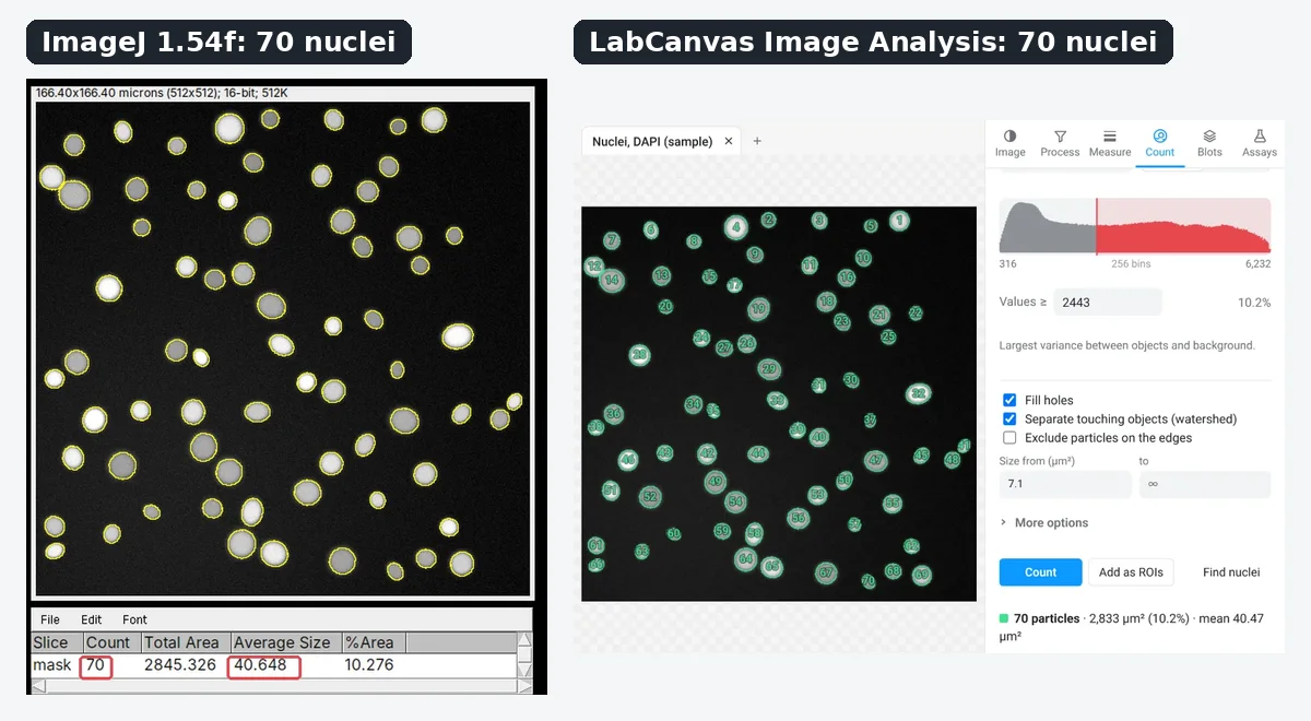
Each pair shows ImageJ first and LabCanvas second, on the same image. The numbers in the captions are what each program reported.
1. Count cells or nuclei
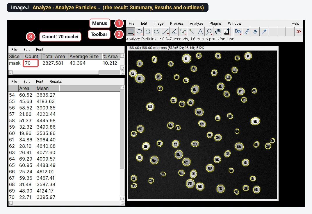
In ImageJ: Image › Type › 8-bit, Image › Adjust › Threshold… (Otsu, Dark background, Apply), Process › Binary › Fill Holes, Process › Binary › Watershed, then Analyze › Analyze Particles… with Size 7-Infinity µm², Show Outlines and Summarize. Six steps; the full walk-through is in how to count cells in ImageJ.
In LabCanvas: open the image, go to the Count tab and click Find nuclei (Otsu, fill holes, watershed and a minimum size in one click), or set them in Count particles and click Count.
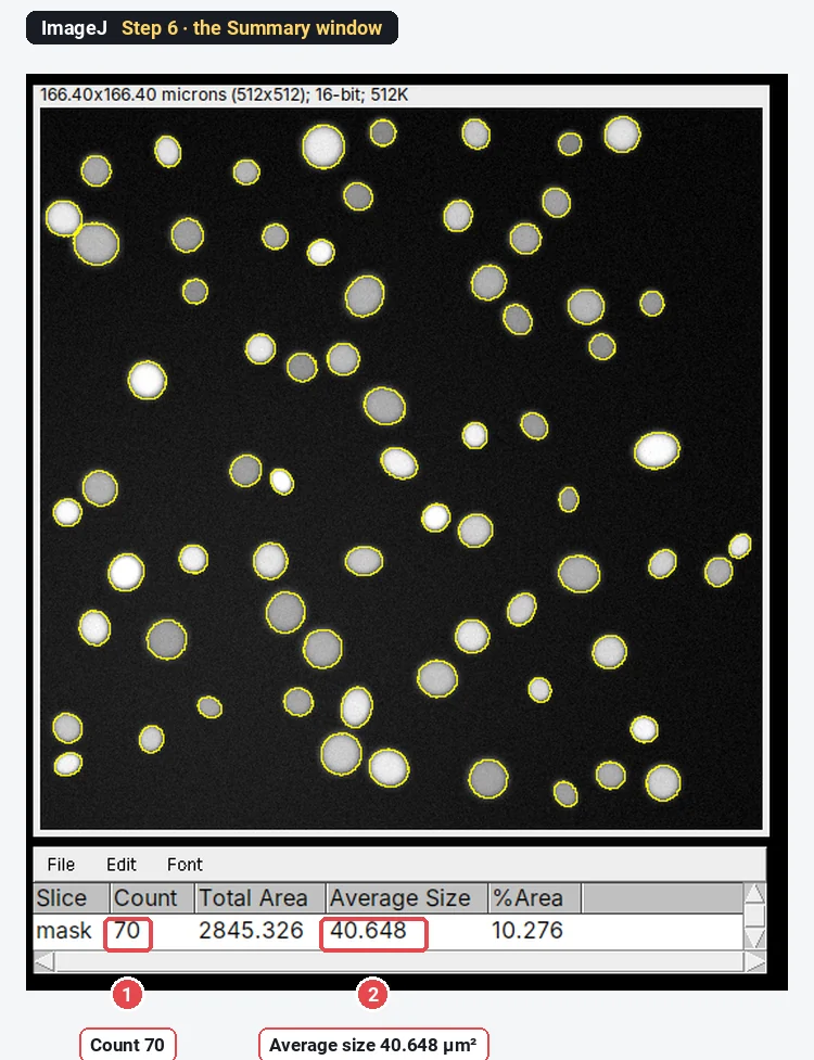
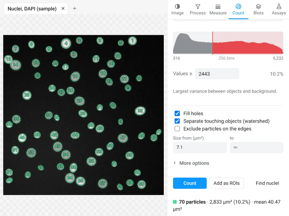
Result: both count all 70 nuclei. The mean areas differ by 0.4% because ImageJ thresholds an 8-bit copy and LabCanvas the raw 16-bit values, so the outlines sit a fraction of a pixel apart. Verdict: a tie on accuracy; LabCanvas is one click instead of six commands, ImageJ is the one you can turn into a macro.
2. Particle size distribution (TEM nanoparticles)
In ImageJ: check the scale in Image › Properties…, threshold (Otsu, Dark background off), Apply, Fill Holes, Watershed, tick Area and Feret's diameter in Analyze › Set Measurements…, run Analyze Particles (20-Infinity nm², Exclude on edges), then Analyze › Distribution… on the Feret column. See nanoparticle size distribution from TEM.
In LabCanvas: tick Area and Feret's diameter in Measure › Set measurements; in Count › Count particles choose Otsu, Dark objects, Fill holes, watershed and Exclude particles on the edges, smallest 20 nm²; click Count, then Send to Graphs with the Feret column for the histogram.
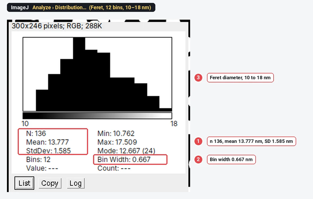
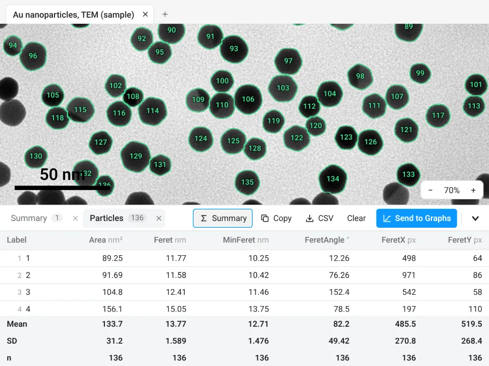
Result: 136 particles in both; mean Feret 13.777 against 13.77 nm. Verdict: a tie on the numbers. ImageJ draws the histogram in its Distribution window; LabCanvas sends the column to Graphs for the histogram and statistics.
3. Western blot densitometry
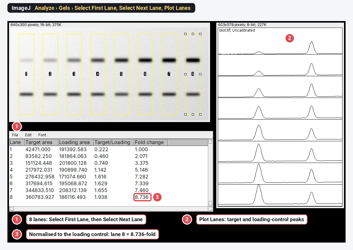
In ImageJ: draw a rectangle on lane 1 and press 1 (Analyze › Gels › Select First Lane), move it to each other lane and press 2, press 3 to plot the lanes, close each peak with a straight line, click inside it with the wand, then divide target by loading control and by lane 1 in a spreadsheet. See western blot quantification in ImageJ.
In LabCanvas: in the Blots tab click Find lanes and Find bands, name the bands, choose the loading control in Normalise to, and click Quantify: the table has area, relative, normalised and fold-change columns.
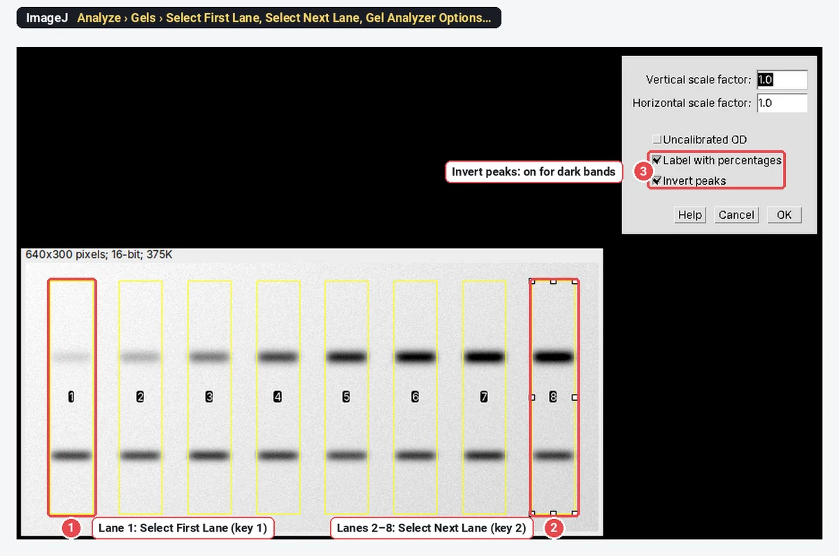
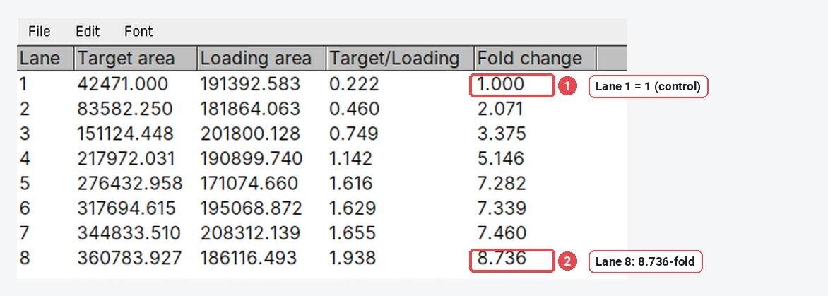
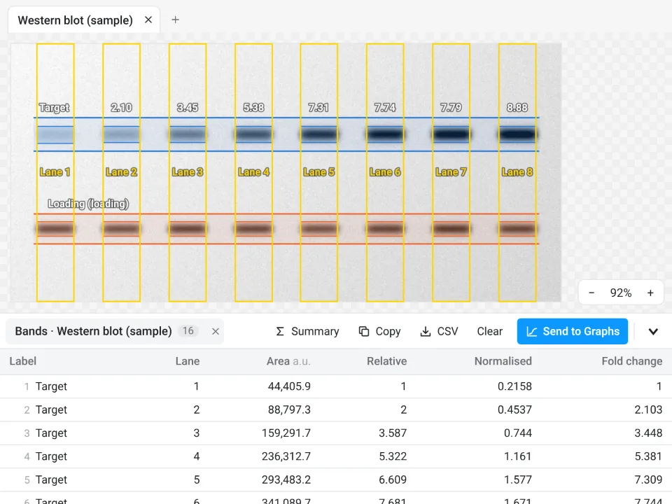
Result: the true lane-8 ratio of this synthetic blot is 8.935-fold; ImageJ gives 8.736 and LabCanvas 8.885. The difference is where each baseline is drawn under the peaks, which matters more than the program. Verdict: LabCanvas is faster and does the normalisation for you; ImageJ gives you full manual control of every baseline.
4. Set the scale and add a scale bar
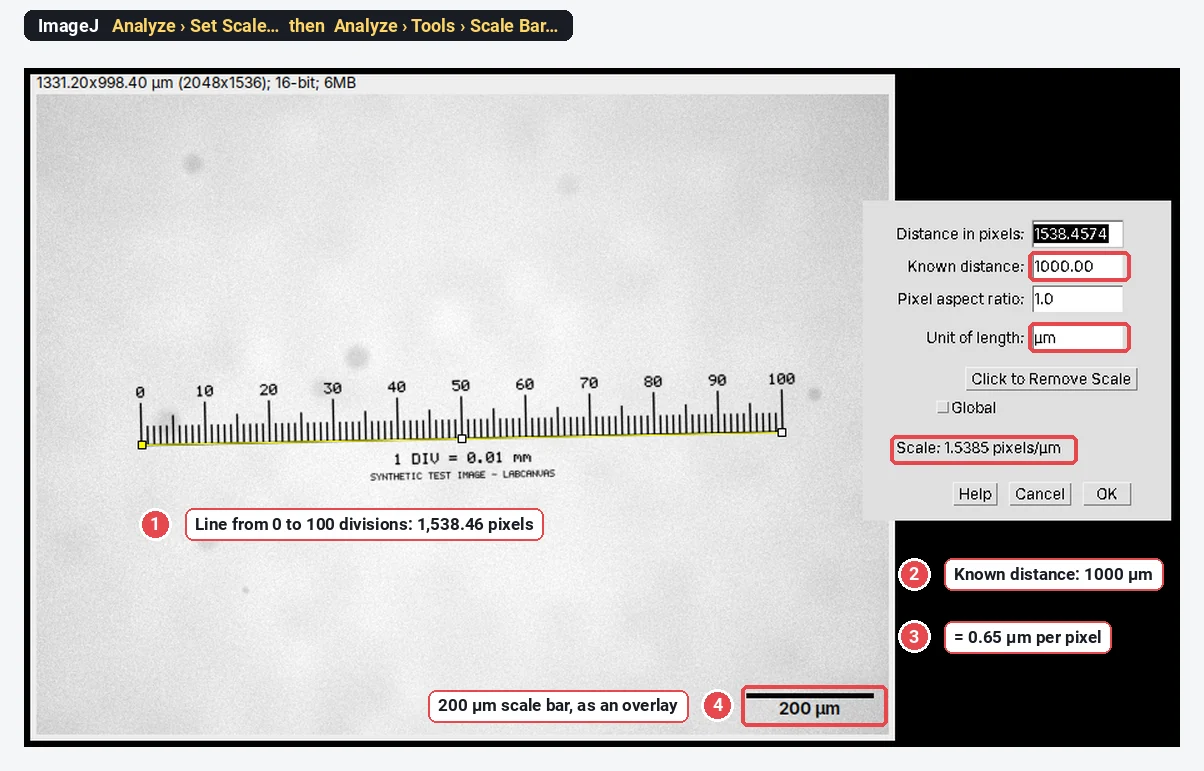
In ImageJ: draw a line along a stage micrometer, Analyze › Set Scale… with the known distance and unit, then Analyze › Tools › Scale Bar…. See how to add a scale bar in ImageJ.
In LabCanvas: draw the same line, then in Image › Scale type the Known distance, choose the unit and click Set scale; tick Scale bar and set its length, position and colour. A pixel size read from the file is used automatically.
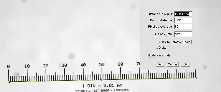
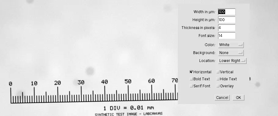
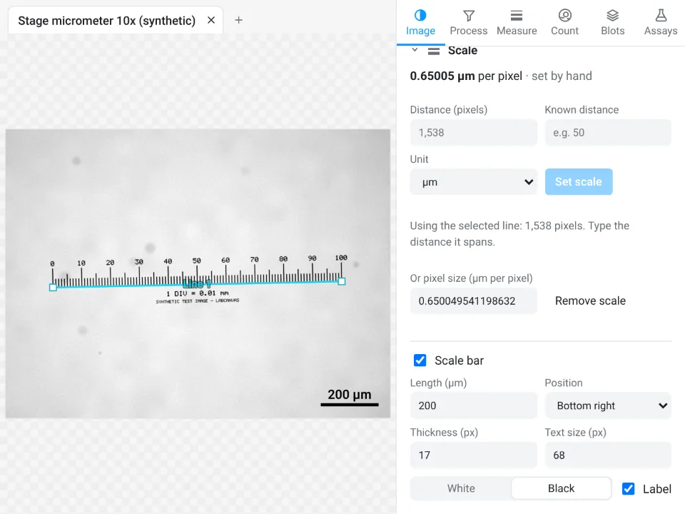
Result: 0.65001 µm per pixel in ImageJ, 0.65005 in LabCanvas, a 0.006% difference from where the line ends were placed. Verdict: equivalent. In both, keep the scale bar on a copy (or as an overlay) and measure the original.
5. Colocalisation (Pearson and Manders)
In ImageJ: plain ImageJ 1.x has no colocalisation command. Fiji's Analyze › Colocalization › Coloc 2 computes Pearson's r and Manders' coefficients with Costes automatic thresholds (Costes et al. 2004); JACoP is another plugin. The ImageJ picture below uses the macro from our colocalisation guide with Coloc 2's thresholds.
In LabCanvas: Measure › Colocalisation: choose the two channels and the region, keep Costes (auto) thresholds and click Calculate; Show colocalised marks the pixels above both thresholds in yellow.
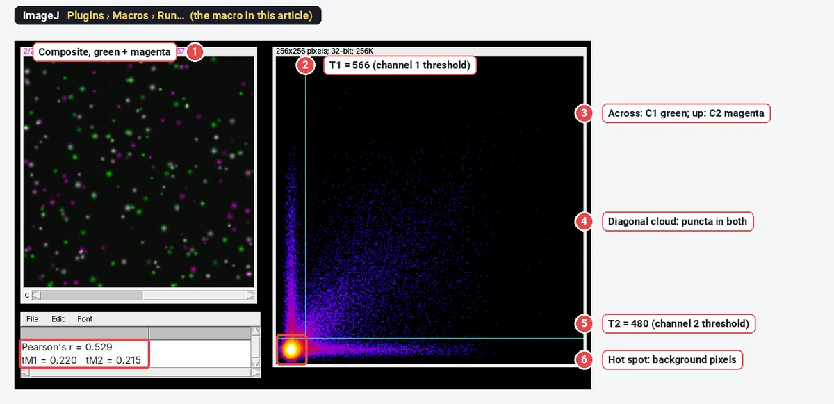
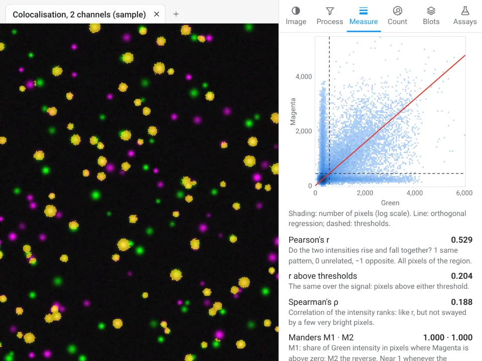
Result: the same Pearson's r; thresholded Manders within 0.001. Verdict: Fiji's Coloc 2 and LabCanvas both do it in one dialog; plain ImageJ needs a plugin or a macro. LabCanvas also gives Spearman's ρ, the overlap coefficient and Li's ICQ in the same panel.
6. Fluorescence intensity of a cell (CTCF)
In ImageJ: tick Area, Mean gray value and Integrated density in Analyze › Set Measurements…, outline the cell and three background squares, add each to the ROI Manager and click Measure, then compute CTCF = IntDen − Area × mean background in a spreadsheet. See how to measure fluorescence intensity in ImageJ.
In LabCanvas: draw the cell (here an oval) and three background rectangles; each goes to the ROI list. Area, Mean, Min and max and Integrated density are on by default in Set measurements; click Measure all ROIs. The CTCF subtraction is done in a spreadsheet or in Graphs, as in ImageJ.
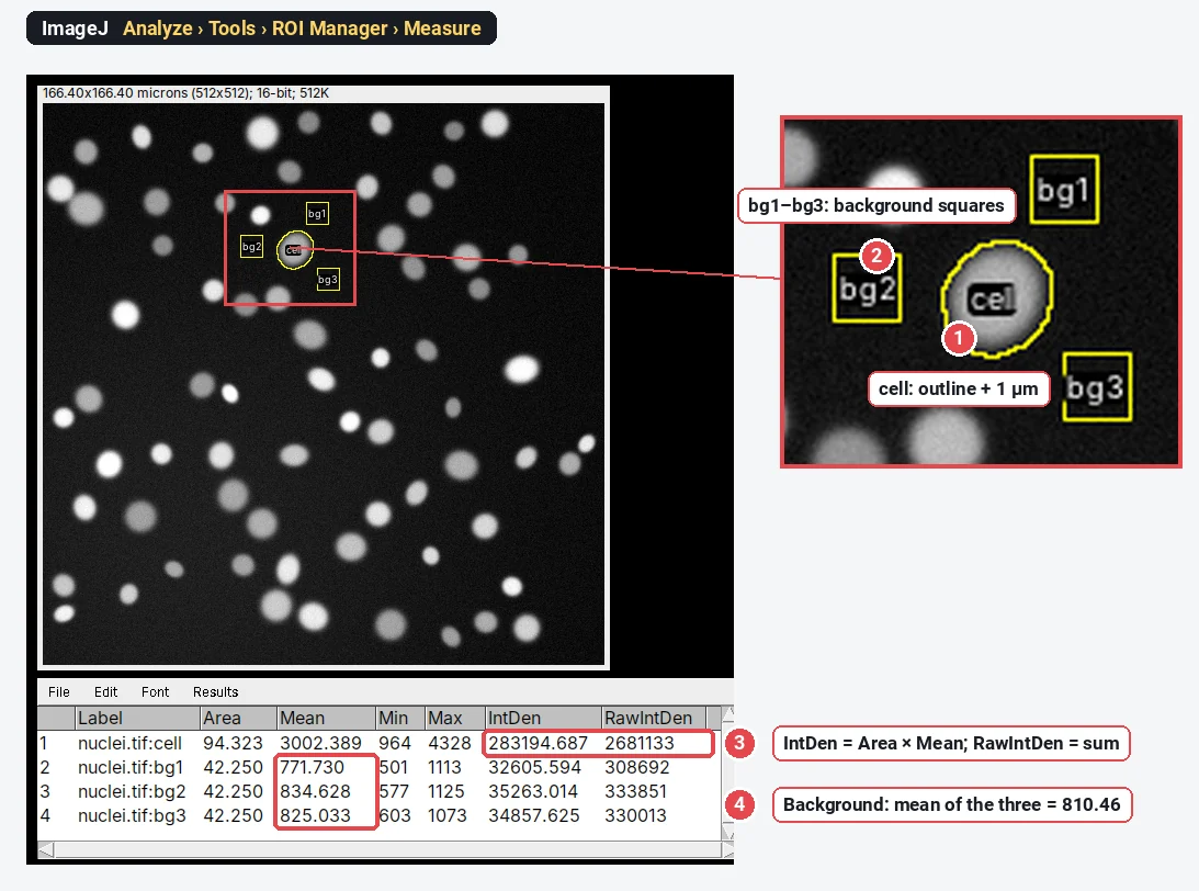
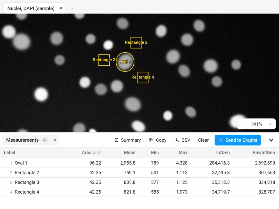
Result:
Six more jobs: the LabCanvas side, and the Fiji route in words
These six were added to LabCanvas in November 2026. The pictures are LabCanvas only, taken from its feature tests. We did not repeat these jobs in Fiji for this article, so the Fiji route is a description, with links to our step-by-step Fiji guides, and there are no ImageJ numbers to compare. The test results quoted are LabCanvas against reference software, not against ImageJ.
7. Repeat an analysis: recipes and ImageJ macros
In Fiji (described): record with Plugins › Macros › Record…, save the macro, then run it on a folder with Process › Batch › Macro…. Macros have variables, loops and conditions and can call any plugin; Fiji also runs scripts in Python (Jython), Groovy, JavaScript and other languages. See ImageJ macros and batch processing.
In LabCanvas: in the Recipe tab click Recording and work as usual: each operation becomes a step you can edit, switch off or reorder. Run on this image, or on open images, Files… or Folder… (with subfolders); the queue is kept in the browser, so a run stopped by closing the tab carries on where it stopped. Under Share, export and ImageJ, download the recipe as an ImageJ macro (.ijm), or paste a macro under Import. Script steps run JavaScript in a worker or Python through Pyodide, and ten built-in recipes (nuclei, percentage area, CTCF per cell, spots, shape, colocalisation and others) are ready to change.
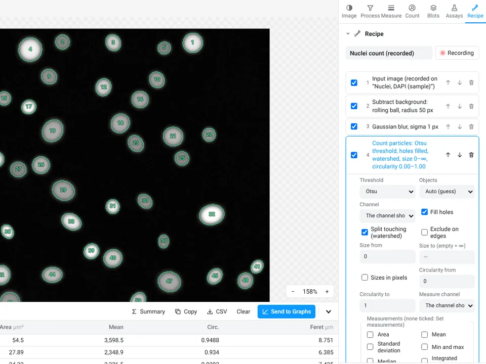
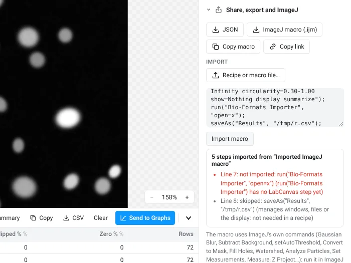
Result: in the tests (95 checks), a replayed recipe gives exactly the tables and pixels of the same operations done one by one, and an exported macro reads back into the same recipe and the same numbers. Limits: only the common commands import (filters, Subtract Background, thresholds, binary operations, Analyze Particles, Set Measurements, Measure, Z Project and a few more); loops, variables, functions and plugin commands do not. There are no plugins, and Python is downloaded from a CDN the first time a Python step runs.
8. Open microscope and DICOM files
In Fiji (described): File › Import › Bio-Formats reads about 150 formats with their metadata, including .czi, .nd2, .lif, .oib, .oir and .lsm; plain ImageJ opens DICOM with File › Open…. See how to open .czi, .nd2 and .lif files in ImageJ and how to open DICOM files in ImageJ.
In LabCanvas: Open an image, or drop the file or a folder. A file that holds several images (a LIF project, CZI scenes, ND2 positions) opens a picker; a folder of DICOM slices opens as one stack per series. The pixel size, Z step, frame interval, channel names and colours come from the file, and files it cannot read say so and how to convert them.
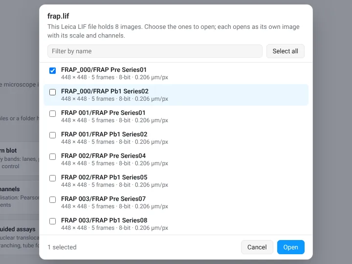
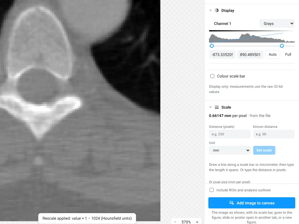
Result: 557 checks on 42 test files against pydicom, readlif, czifile, nd2, oiffile and tifffile. Limits: DICOM in RLE, JPEG lossless and the common uncompressed encodings, not JPEG 2000; CZI uncompressed, Zstd or JPEG, not JPEG XR; ND2 from NIS-Elements 3 on, not the earlier JPEG 2000 files; from a VSI file only the pictures stored inside it, not the full-resolution .ets scan. OIR, LSM, IMS, NDPI, OIF, MRC, DM3/DM4 and other formats that Bio-Formats reads are not read: export them as OME-TIFF.
9. 3D objects in a Z-stack
In Fiji (described): Analyze › 3D Objects Counter labels the objects above a threshold and measures their volume, surface, centroid and intensity; the 3D ImageJ Suite update site adds 3D watershed segmentation and more measurements; Plugins › 3D Viewer renders the stack. See 3D projection and the 3D viewer in ImageJ.
In LabCanvas: Count › 3D objects thresholds the whole stack (ImageJ's methods on the stack histogram), fills holes in 3D, labels 6-, 18- or 26-connected objects and splits touching ones with a 3D watershed that uses the Z step. Each object gets volume, surface, sphericity, centroid, bounding box, intensities per channel, 3D Feret, ellipsoid axes and nearest-neighbour distances, and a second channel can be colocalised by object and by volume. 3D view opens a volume viewer (MIP, volume, isosurface, objects) linked to the table; Send to 3D Studio sends the meshes for rendered pictures.
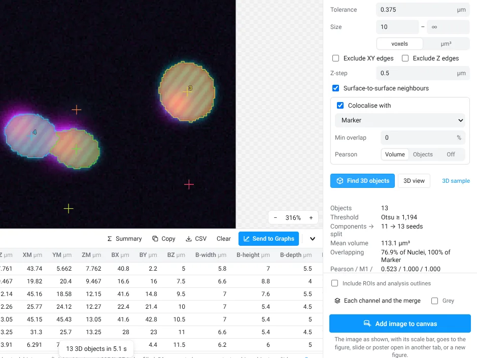
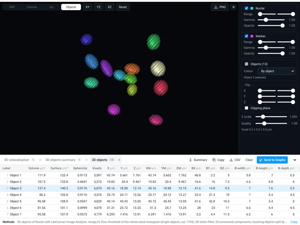
Result: 237 checks against scikit-image and SciPy; on scikit-image's cells3d nuclei, the connected components (21) and the watershed objects (26) match scikit-image's count and volumes. Limits: no 3D tracking and no 3D deep-learning model; the stack must fit in memory.
10. AI nucleus segmentation (StarDist)
In Fiji (described): enable the CSBDeep and StarDist update sites, then Plugins › StarDist › StarDist 2D with the fluorescent-nuclei model (an H&E model is also there); the result is a label image or ROIs to measure. Cellpose runs from Fiji through a wrapper and a Python environment. See StarDist, Cellpose and Weka in Fiji.
In LabCanvas: Count › AI segmentation, model Nuclei, fluorescence (StarDist), then Segment. The model (5.7 MB) is downloaded once and runs on your device; the nuclei become the Count tab's particles, with the same table, Send to Graphs, ROIs, workflows and batch. It is also one of the guided assays.
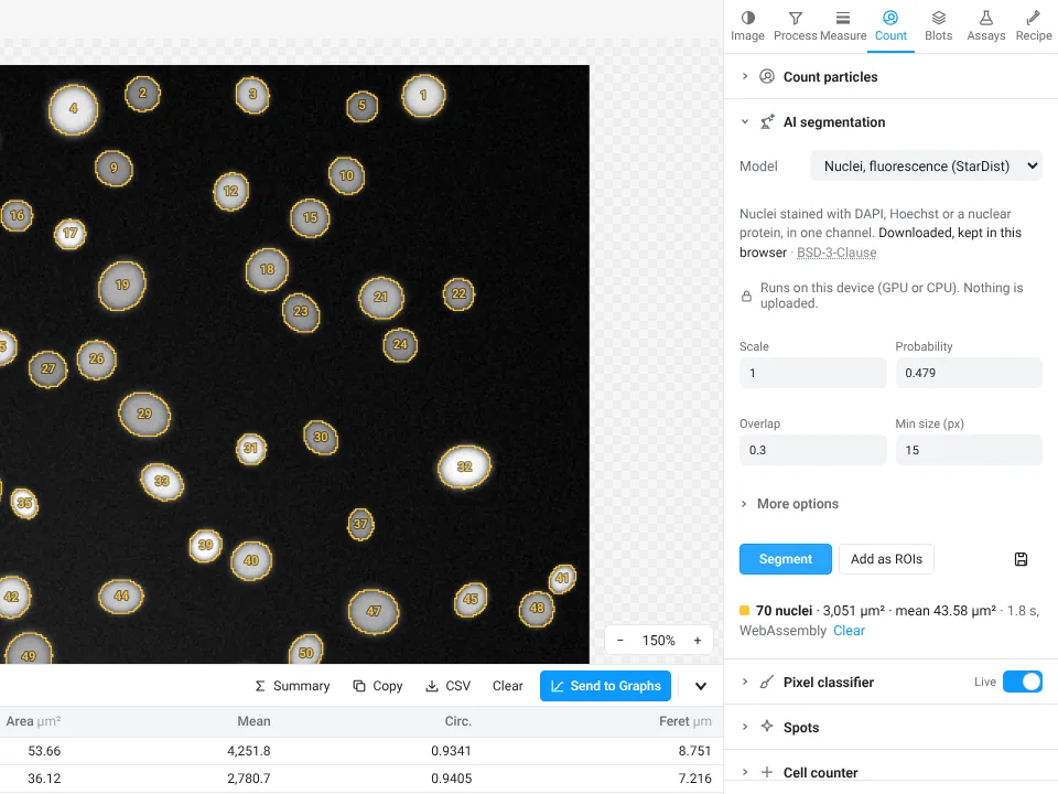
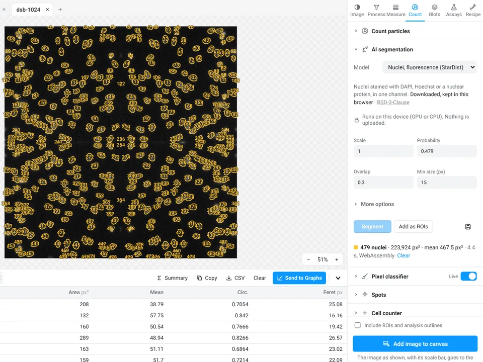
Result: on four test images, including both shown here, LabCanvas finds the same objects as the stardist Python package (F1 1.000, and an intersection over union of at least 0.9 for every matched object). On the nuclei sample it counts the same 70 as the threshold in job 1, with larger outlines (mean 43.58 µm² against 40.47 µm²), so use one method per study. Limits: one model ships, for fluorescent nuclei in 2D. Cellpose works only with a model you convert to ONNX and open yourself: its pretrained weights are licensed for non-commercial use and are not included. There is no H&E model.
11. Deconvolution and tile stitching
In Fiji (described): deconvolve with DeconvolutionLab2 (Plugins › DeconvolutionLab2 › DeconvolutionLab2 Lab), using a PSF from Diffraction PSF 3D or PSF Generator or one measured from beads; stitch with Plugins › Stitching › Grid/Collection stitching, or BigStitcher for data that do not fit in memory. See deconvolution in ImageJ and Fiji and stitching tiles in Fiji.
In LabCanvas: Process › Deconvolve: compute the PSF from the optics (Born & Wolf, Gibson–Lanni or confocal) or measure it from beads, pick Richardson–Lucy, RL with total variation, Wiener or Tikhonov, 2D or the whole stack in 3D, and Preview a crop with a before/after split; it runs on the GPU through WebGPU where the browser has one, otherwise on the CPU. Process › Stitch: a grid (columns, rows, order, overlap), a Fiji TileConfiguration file or OME stage positions; Register finds each overlap by phase correlation and drops links that disagree, then fusion blends the tiles, with flat-field correction.
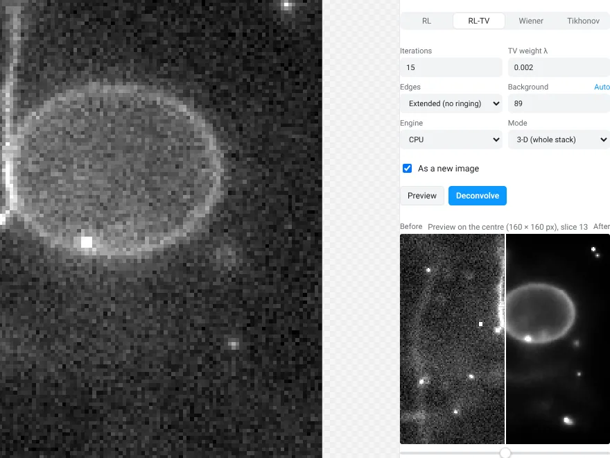
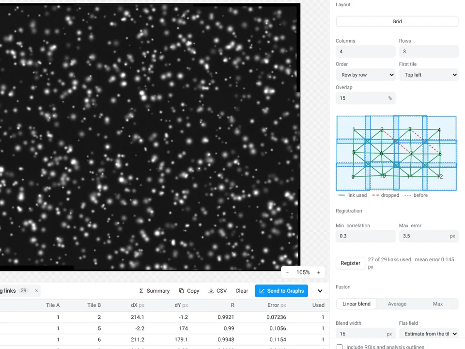
Result: Richardson–Lucy matches scikit-image's richardson_lucy and the PSFs match microscPSF and psfmodels (31 checks); stitched tiles land within half a pixel of their true positions (22 checks). Limits: fewer algorithms than DeconvolutionLab2, and the tiles to stitch must fit in memory together.
12. Very large images and whole slides
In Fiji (described): Bio-Formats can open a large file as a virtual stack or one resolution level of a pyramid, and BigDataViewer browses data bigger than memory; for analysis across whole slides most labs use QuPath (see CellProfiler vs QuPath vs ImageJ).
In LabCanvas: open a pyramidal OME-TIFF, an Aperio SVS, a BigTIFF or a large ImageJ stack, or an OME-Zarr folder or web address: it opens as a large image, and only the tiles in view are read, with a minimap and a scale bar. To measure, Work on region reads a rectangle, the view or the whole image at a chosen resolution level, and a range of slices and frames, into a normal image (up to 600 million values) that every tool works on, with the level's pixel size.
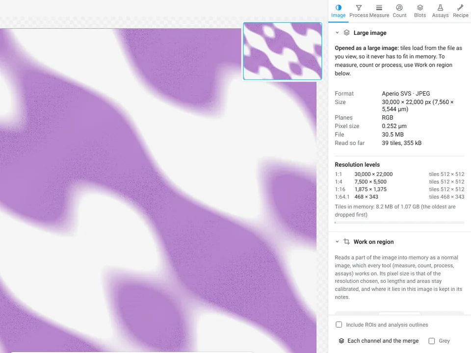
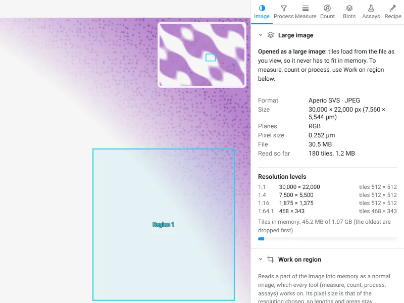
Result: 156 checks against tifffile, zarr, numcodecs and libjpeg-turbo. Limits: SVS files with JPEG 2000 tiles cannot be read (convert them once with QuPath, bfconvert or vips); measurements run on a region, not on the whole slide at full resolution, and batch runs, assays and stitching need a region first.
Where ImageJ and Fiji are better
- Plugins. Hundreds of them, for almost any measurement a lab has needed: TrackMate, Coloc 2, Bio-Formats, the 3D ImageJ Suite, MorphoLibJ, BigStitcher, Trainable Weka Segmentation, StarDist, deepImageJ and many more through the Fiji updater. The ecosystem is far larger than anything LabCanvas has built in, and LabCanvas has no plugins at all.
- Macros and scripts. The macro language has variables, loops and conditions and can call any plugin, and Fiji's scripts (Python/Jython, Groovy, JavaScript and others) reach everything in it, on thousands of images. A LabCanvas recipe imports only the common commands of a macro.
- Time-lapse and 3D. TrackMate tracks in 2D and 3D with many detectors and linkers and is far more complete than LabCanvas's 2D tracking assay; registration, 3D plugins and BigDataViewer cover more than LabCanvas's 3D objects panel.
- Deep-learning segmentation. Fiji runs StarDist with fluorescence and H&E models, Cellpose with its pretrained models, and BioImage Model Zoo models through deepImageJ; LabCanvas ships one model, StarDist for fluorescent nuclei.
- File formats. Bio-Formats reads about 150 formats, including .oir, .lsm, .ims and .ndpi, which LabCanvas cannot open, and the CZI, ND2 and SVS variants LabCanvas turns away (JPEG XR, JPEG 2000).
- Big data. With enough memory, virtual stacks, BigDataViewer, BigStitcher and a workstation, Fiji works on datasets that would not fit in a browser tab; LabCanvas views such images tile by tile but measures a region at a time.
- Open source, offline and free. You can read every line of the code, cite a paper that thousands of studies cite, and find a forum answer for almost any problem. It works offline, is free and needs no account.
Where LabCanvas is better
- Nothing to install. No Java, no plugin hunting, no update sites: it opens in a browser on a laptop, a locked-down institute computer or a tablet.
- Guided, not assembled. Each job is one panel with settings that work in one click and a live preview, so the order of commands is not something you have to know. Twelve assays that need plugins or macros in ImageJ are built in, each with a sample image to practise on.
- Heavier jobs without setup. StarDist, 3D objects, deconvolution, stitching and the microscope and DICOM readers are built in: no update sites to enable, no Python environment and nothing to install on a shared computer.
- Recipes that go both ways. Work once with the recorder on, run the recipe on a folder, and export it as an ImageJ macro so a colleague can repeat the steps in Fiji.
- Checks before you measure. The image check flags clipped pixels, JPEG compression, pixels copied from a figure, gaps in the histogram left by earlier processing, uneven illumination and focus.
- Raw values by default. Thresholds and measurements always read the 8-, 16- or 32-bit data, never the displayed picture, so contrast changes or an 8-bit conversion cannot creep into the numbers.
- From numbers to a figure. Send to Graphs for statistics and plots, images with their scale bar and ROIs straight into a figure, slide or poster, and a methods sentence with every table.
- Validated in the open. 5,144 automated checks against scikit-image, SciPy, NumPy, pydicom, tifffile, the stardist package and images with known answers, with the tolerances published on the validation page.
Which should I use?
| Your situation | Use |
|---|---|
| A standard measurement on a few images, and no time to learn ImageJ | LabCanvas |
| You cannot install software, or you are on a tablet | LabCanvas (or ImageJ.JS for ImageJ itself) |
| A guided assay: translocation, foci, colonies, wound, FRAP, calcium, tracking, Sholl, tubes | LabCanvas, or Fiji with the matching plugin or macro |
| Teaching a class the basics of measuring images | Either; LabCanvas needs no installation on student computers |
| The same standard steps on a folder of images | Either: a LabCanvas recipe, or Fiji with a macro |
| Thousands of images, or a pipeline with loops, conditions or plugin calls | Fiji with a macro or script (or CellProfiler) |
| A method that needs a specific plugin (TrackMate, MorphoLibJ, BigStitcher, deepImageJ…) | Fiji |
| Fluorescent nuclei that a threshold cannot separate | Either: StarDist in LabCanvas or in Fiji |
| H&E nuclei, or cells with pretrained Cellpose models | Fiji |
| 3D objects, deconvolution or stitching with standard settings | Either; LabCanvas needs no setup, Fiji has more options |
| Tracking in 3D, or time-lapse data too large for memory | Fiji |
| .czi, .nd2, .lif, .oib or DICOM files | Either (check the limits in job 8) |
| .oir, .lsm, .ims, .ndpi or another format LabCanvas cannot read | Fiji, through Bio-Formats |
| Viewing a whole-slide image and measuring regions of it | Either; for analysis across whole slides, QuPath |
| Working offline, or with open-source software only | ImageJ or Fiji |
| A published protocol written for ImageJ | ImageJ or Fiji, to follow it exactly |
Many people will use both: Fiji for the unusual jobs and anything that needs a plugin, LabCanvas for the everyday ones, the common heavier ones without setup, and turning results into figures. Pick one per study so every image is measured the same way.
Reporting it
Whichever you use, name the program and version, the settings and the pixel size:
Nuclei were counted in [ImageJ 1.54f / Fiji] ([Otsu] threshold, Fill Holes, Watershed, Analyze Particles with a minimum area of [7 µm²]) at [0.325] µm per pixel (Schneider et al. 2012).
Images were analysed in LabCanvas Image Analysis (www.labcanvas.com, accessed [month year]). [Paste the methods sentence of the results table, which names the threshold method, size range and pixel size.]
More in how to cite ImageJ and Fiji.
Try it on the same images
Open Image Analysis and click a sample on the start screen (the nuclei, the western blot or the two channels) to repeat jobs 1, 3, 5 and 6 above, and Count › AI segmentation on the nuclei for job 10; Count › 3D objects has a 3D sample for job 9, and every assay has its own sample under Assays. It is free with a LabCanvas account (downloading files is part of LabCanvas Pro). The complete guide goes through every tool. ImageJ and Fiji are independent open-source projects; LabCanvas is not affiliated with them.
References
- Costes SV, Daelemans D, Cho EH, Dobbin Z, Pavlakis G, Lockett S (2004). Automatic and quantitative measurement of protein-protein colocalization in live cells. Biophysical Journal 86(6): 3993–4003. doi:10.1529/biophysj.103.038422
- Linkert M, Rueden CT, Allan C, et al. (2010). Metadata matters: access to image data in the real world. Journal of Cell Biology 189(5): 777–782. doi:10.1083/jcb.201004104
- Schindelin J, Arganda-Carreras I, Frise E, et al. (2012). Fiji: an open-source platform for biological-image analysis. Nature Methods 9(7): 676–682. doi:10.1038/nmeth.2019
- Schneider CA, Rasband WS, Eliceiri KW (2012). NIH Image to ImageJ: 25 years of image analysis. Nature Methods 9(7): 671–675. doi:10.1038/nmeth.2089
- ImageJ disclaimer (public domain status of ImageJ 1.x): imagej.net/ij/disclaimer.html
- LabCanvas Image Analysis validation: labcanvas.com/image-analysis-validation
Frequently asked questions
Is there an alternative to ImageJ?
Yes, several. Fiji is ImageJ with plugins bundled and is the usual upgrade. CellProfiler is built for batches of thousands of images, QuPath for whole slide images, and napari and ilastik for Python and machine-learning workflows. For everyday measurements in a browser with nothing to install, LabCanvas Image Analysis uses ImageJ's measurement names and definitions and adds guided assays. None of them replaces the whole ImageJ plugin ecosystem.
Is ImageJ free?
Yes. ImageJ 1.x was written at the US National Institutes of Health and is in the public domain, and Fiji is a free, open-source distribution of it. Both run on Windows, macOS and Linux. LabCanvas Image Analysis is free with a LabCanvas account; downloading files (CSV, TIFF, PNG) is part of LabCanvas Pro.
Can I count cells online without ImageJ?
Yes. In LabCanvas Image Analysis, open the image in the browser, go to the Count tab and click Find nuclei (Otsu threshold, fill holes, watershed and a minimum size in one click), or set the threshold and size range yourself in Count particles. On the synthetic nuclei sample it counts 70 nuclei, the same as ImageJ. The image is measured inside the browser tab, not uploaded to a server.
Will LabCanvas give me the same numbers as ImageJ?
For standard measurements, nearly: they follow ImageJ's definitions (Area, Mean, IntDen, RawIntDen, Feret, the same 16 automatic threshold methods). On the samples in this article the counts were identical and the means agreed within about 1 to 2%; the small differences come from where a band baseline or an outline is drawn. Use one program for a whole study and report its settings.
Can LabCanvas run ImageJ macros or plugins?
Not plugins, and not every macro. A LabCanvas recipe can import the common ImageJ macro commands (filters, Subtract Background, thresholds, binary operations, Analyze Particles, Set Measurements, Measure, Z Project and others) and lists every line it cannot import, such as loops, variables and plugin commands. A recipe also exports as an .ijm macro to run in ImageJ or Fiji, and script steps run JavaScript or Python (through Pyodide). If your analysis depends on a Fiji plugin (TrackMate, MorphoLibJ, the 3D ImageJ Suite, BigStitcher and others) or on a long macro with loops and variables, stay with Fiji.
Can LabCanvas open .czi, .nd2 or .lif files?
Yes, with limits. It opens Leica LIF, Zeiss CZI (uncompressed, Zstd or JPEG, not JPEG XR), Nikon ND2 (not the early JPEG 2000 files), Olympus OIB, the pictures stored inside a VSI file (not the full-resolution .ets scan) and DICOM, as well as TIFF, OME-TIFF, BigTIFF, Aperio SVS and OME-Zarr. Scale, Z step, frame interval and channel names come from the file. It does not read OIR, LSM, IMS, NDPI and many other formats that Fiji reads through Bio-Formats (about 150 in all): export those as OME-TIFF, or use Fiji.
Does LabCanvas have StarDist or Cellpose?
It runs StarDist's 2D_versatile_fluo model for fluorescent nuclei on your own device (on the GPU through WebGPU, or the CPU); on four test images it found the same objects as the stardist Python package. Cellpose works only with a model you convert to ONNX and open yourself, because the pretrained Cellpose weights are licensed for non-commercial use only and are not included. There is no model for H&E images. In Fiji, the StarDist plugin also has an H&E model, and Cellpose runs with its pretrained models.
Can I use ImageJ on an iPad or a Chromebook?
There is no ImageJ app for iPad or Android. ImageJ.JS runs ImageJ 1.x inside a browser, more slowly than on the desktop, and Fiji can be used on an institutional server through a remote desktop. LabCanvas Image Analysis is built for the browser and works on a tablet.
Which one should I cite in a paper?
Cite the software you measured with. For ImageJ, Schneider, Rasband and Eliceiri 2012 (Nature Methods 9:671); for Fiji, Schindelin et al. 2012 (Nature Methods 9:676). For LabCanvas, name LabCanvas Image Analysis, www.labcanvas.com and the month you used it, then paste the methods sentence that comes with each results table.
Try it in LabCanvas
Every app is free to start in your browser. Create an account and begin.
Start Image Analysis free in your browserKeep reading
How to use ImageJ: a beginner's tutorial for the 10 everyday jobs (2026)
How to use ImageJ and Fiji: get started, open an image, then 10 everyday jobs (scale, measure, threshold, count, background, blots) with exact menu paths.
How to set the scale and add a scale bar in ImageJ (with a calibration image to practise on)
Set the scale in ImageJ (Analyze › Set Scale) from a micrometer, scale bar or pixel size, add a scale bar, and practise on a free calibration image.
Western blot quantification in ImageJ, step by step (and the 3-click way)
Quantify a western blot in ImageJ with Analyze › Gels, normalise to a loading control or total protein, and get fold change. Plus a 3-click way.