How to count cells in ImageJ (automatic and manual)
Count cells in ImageJ: automatic (threshold, Watershed, Analyze Particles) or manual (Cell Counter, Multi-point), plus cells per mm² and % positive.
Contents
To count cells automatically in ImageJ, convert the image to 8-bit, set a threshold with Image › Adjust › Threshold…, clean up the mask with Process › Binary (Convert to Mask, Fill Holes, Watershed), then run Analyze › Analyze Particles… with a size and circularity range and Summarize ticked: the Summary window gives the count. To count by hand, use Plugins › Analyze › Cell Counter in Fiji, or the counters of the Multi-point tool in plain ImageJ 1.x.
Automatic counting works best on stained nuclei (DAPI, Hoechst) and other fluorescent cells on a dark background. Unstained cells in brightfield or phase contrast are much harder, and this guide says what to do instead.
Which method fits your image
| Your image | The route that works |
|---|---|
| Fluorescent nuclei or cells, mostly apart | Automatic: threshold, watershed, Analyze Particles |
| Crowded, touching nuclei | Automatic with watershed; for dense tissue, StarDist or Cellpose |
| Small bright cells or spots where only the number matters | Find Maxima |
| Unstained cells in brightfield or phase contrast | A trained pixel classifier, a deep-learning tool, or counting by hand |
| A few images, or cells you must judge by eye (shape, two markers) | Manual: Cell Counter or the Multi-point tool |
| Cells in a hemocytometer, for cells per mL | Count the cells in each large square, then use the hemocytometer calculator |
| Bacterial or yeast colonies on a plate | A colony counter: see colony counting with ImageJ |
Automatic counting in ImageJ (or Fiji)
These commands are part of ImageJ 1.x, so they are the same in plain ImageJ and in Fiji.
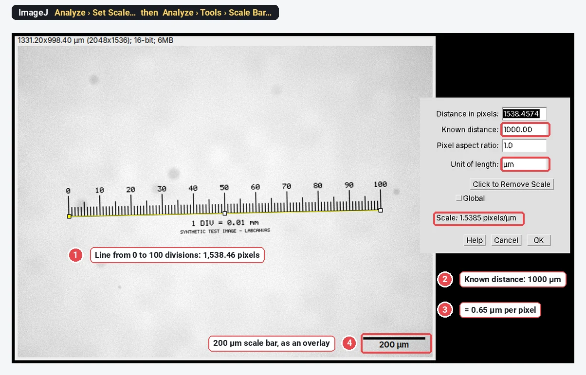
- Set the scale with Analyze › Set Scale… if the file does not carry it, so that sizes come out in µm²; see how to set the scale in ImageJ.
- Keep one channel: for a multi-channel image, use Image › Color › Split Channels and keep the nuclear channel. Then Image › Type › 8-bit. That is fine for counting; measure intensities on the original file.
- Smooth and flatten, if needed: Process › Filters › Gaussian Blur… with a sigma of 1 or 2 pixels evens out noise, and Process › Subtract Background… removes a bright corner or a gradient.
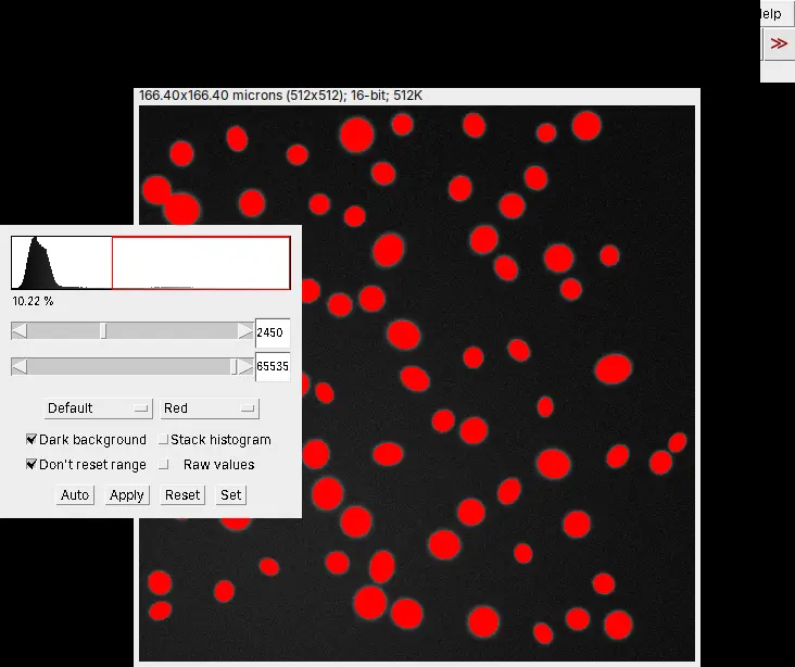
- Threshold: open Image › Adjust › Threshold…, pick a method (Default, Otsu, Li, Triangle and others), tick Dark background for fluorescence, and check that the red overlay covers every nucleus and nothing else. Click Apply. The methods are compared side by side in ImageJ threshold methods, with pictures.
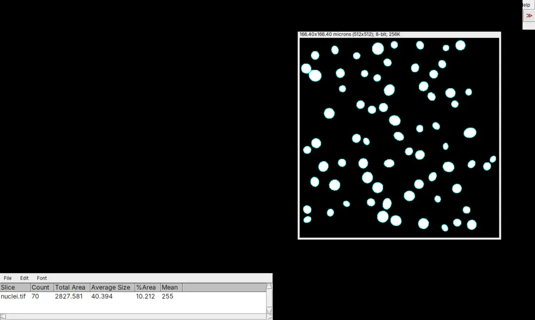
- Clean up the mask: Process › Binary › Convert to Mask (if Apply did not already make one), then Process › Binary › Fill Holes and Process › Binary › Watershed, which cuts touching round objects apart with one-pixel lines.
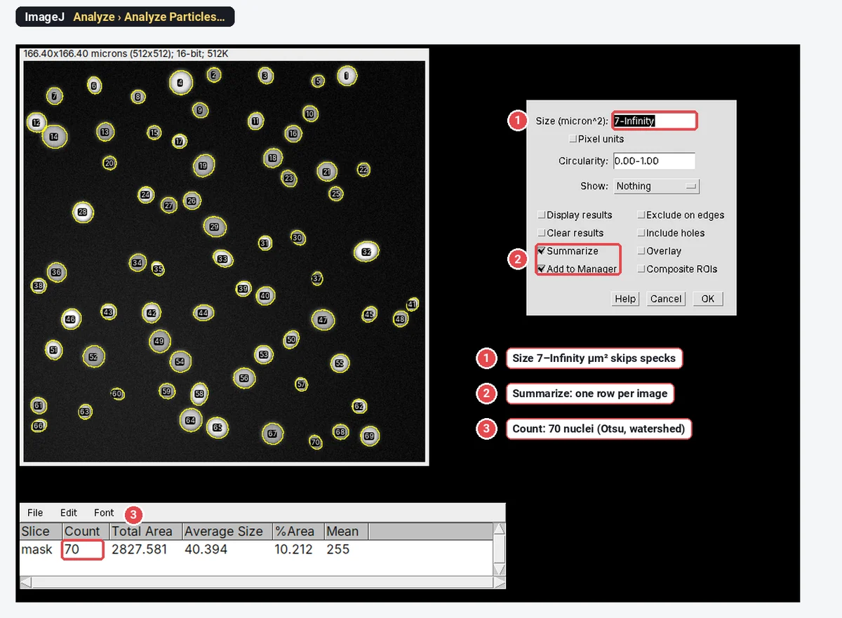
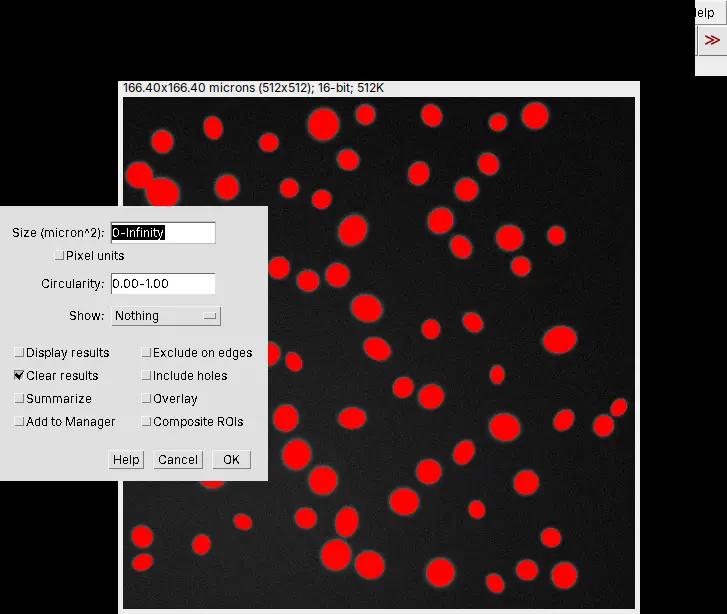
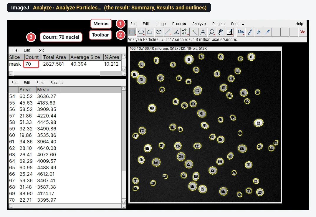
- Count: run Analyze › Analyze Particles… with the settings below, then read Count in the Summary window, which also gives Total Area, Average Size and %Area.
| Analyze Particles setting | What to choose |
|---|---|
| Size (µm² once the scale is set) | A lower limit that drops debris, for example a fifth of a typical nucleus's area, up to Infinity |
| Circularity | 0.00–1.00 keeps everything; raise the lower limit to drop long debris and scratches |
| Show | Outlines or Overlay, so you can check what was counted |
| Display results, Summarize | Ticked: one row per cell, and the count |
| Exclude on edges | Ticked for measurements per cell; for density, see below |
| Include holes | Ticked, so a nucleus with a dim centre is measured whole, not as a ring |
| Add to Manager | Ticked if you want to measure each cell in another channel afterwards |
Before you trust the number, lay the outlines over the image and look: a merged pair, a split cell or a counted speck is easy to see there and invisible in the Summary. Every option in the dialog is explained in Analyze Particles, explained.
Only the number? For small, round, bright cells, Process › Find Maxima… counts one point per peak without making a mask: set Prominence > until each cell gets one point, tick Exclude edge maxima if you need to, and choose Output type: Count.
Manual counting: Cell Counter (Fiji) or the Multi-point tool (ImageJ 1.x)
Counting by hand is still the reference when cells touch, when you classify them by eye, or when you check an automatic count.
In Fiji: Plugins › Analyze › Cell Counter
- Open the image, then Plugins › Analyze › Cell Counter › Cell Counter.
- Click Initialize.
- Select a counter type (Type 1, Type 2 and so on; you can add more) and click each cell. A numbered marker of that type appears on each one.
- Click Results for the counts of every type (for a stack, per slice and in total).
Plain ImageJ 1.x does not include the Cell Counter plugin.
In plain ImageJ 1.x: the Multi-point tool and its counters
- Right-click the point tool in the toolbar and choose Multi-point Tool.
- Double-click the tool (or use Edit › Options › Point Tool…) and choose a Counter: 0 for the first class of cell, 1 for the second, and so on. The dialog shows the count for the current counter.
- Click each cell. Alt-click (or Ctrl-click) a point to remove it.
- Analyze › Measure lists every point with its counter; Alt+Y shows the counts per counter in a table.
The ImageJ wiki notes that the Multi-point tool now does most of what Cell Counter does, so you do not need Fiji just to count by hand.
Cells per mm² and percent positive
Density. Cells per mm² = the count ÷ the area of the field in mm². The field area is the width × the height in pixels × the pixel size squared. The built-in nuclei sample used below is 512 × 512 pixels at 0.325 µm per pixel: 166.4 µm square, or 0.0277 mm². Its 70 nuclei are about 2,530 nuclei per mm².
For density, do not simply exclude the cells cut by the edge, or you undercount: either count them all, or use a counting frame (keep the cells touching two chosen edges, drop those touching the other two). For cells per mL from a hemocytometer, the mean count per large square × 10,000 × the dilution gives cells/mL; the hemocytometer calculator does the sums, with viability and seeding volumes.
Percent positive
When a threshold cannot separate the cells
Uneven staining, textured cells and brightfield or phase-contrast images defeat a single threshold. In Fiji, Plugins › Segmentation › Trainable Weka Segmentation lets you paint a few strokes on each class (cell and background to start); a random forest then classifies every other pixel, and you paint more where it is wrong. Create result gives a class image you threshold and count with Analyze Particles as above (Arganda-Carreras et al. 2017).
Be realistic with unstained cells: a classifier helps when cells differ from the background in texture or colour, but cells that touch with no visible boundary still merge. For those, deep-learning segmentation such as Cellpose (Stringer et al. 2021) or StarDist, which run in Python or as Fiji plugins, or counting by hand, is the honest answer.
Pitfalls
- Merged and split cells. Watershed separates touching round nuclei, but it also cuts long or bent cells in two. Compare the outlines with the image, and leave watershed off for elongated cells; watershed for touching particles shows both cases.
- Debris and noise counted as cells. Set a minimum size (a fifth of a typical nucleus works for most nuclear stains), blur slightly before thresholding, and use circularity to drop scratches.
- Uneven illumination. One threshold for a field that is brighter on one side picks up background there and misses dim cells elsewhere. Subtract the background first (Process › Subtract Background…), or train a classifier.
- A different threshold for every image. Choose the method once, on a few representative images, and use the same settings for every image in the experiment; adjusting each image towards the answer you expect biases the result.
- An inverted mask. One huge particle, or a count of holes, means the background became the object: check Process › Binary › Options › Black background, or invert the mask.
- Nuclei are not always cells. Multinucleated cells, dividing cells and apoptotic fragments break the one-nucleus-one-cell rule; say what you counted.
- Never checked against a human. Count three to five fields by hand and compare them with the automatic count before you run hundreds of images.
Reporting it
A methods sentence to copy, with the parts in brackets filled in:
Nuclei were counted in [Fiji (ImageJ 1.54)] on [DAPI] images ([n] fields per well, [20×] objective, [0.325] µm per pixel): [Otsu] threshold, Fill Holes and Watershed, then Analyze Particles with a size range of [7 µm²] to infinity and circularity [0.30–1.00]. Counts were converted to nuclei per mm² using the field area ([0.0277] mm²). Nuclei were scored [Ki-67]-positive when their mean intensity exceeded [a cut-off set on the secondary-antibody-only control].
Cite ImageJ (Schneider et al. 2012) or Fiji (Schindelin et al. 2012), and name the threshold method; Otsu's method is Otsu (1979).
To show the result, plot cells per mm² or percent positive for each condition with every biological replicate (well, animal or independent experiment) as a point, not every field, and the mean ± SD. For the figure, Image › Overlay › Flatten burns the outlines into an RGB copy, and Analyze › Tools › Scale Bar… adds the scale bar.
An easier way: count cells in LabCanvas
The same count runs in the browser in LabCanvas Image Analysis, with nothing to install and no plugins.
- Open your TIFF, or click the nuclei sample on the start screen.
- Go to the Count tab.
- Click Find nuclei for the one-click route (Otsu threshold, holes filled, touching nuclei split, specks under a fifth of the typical nucleus left out), or set the threshold, Fill holes, Separate touching objects (watershed) and the size range yourself in Count particles and click Count.
- Read the Summary row (Count, Total Area, Average Size, %Area, Mean); for clicking by hand, the Cell counter in the same tab counts in up to 20 named categories with their percentages.
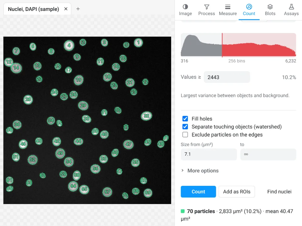
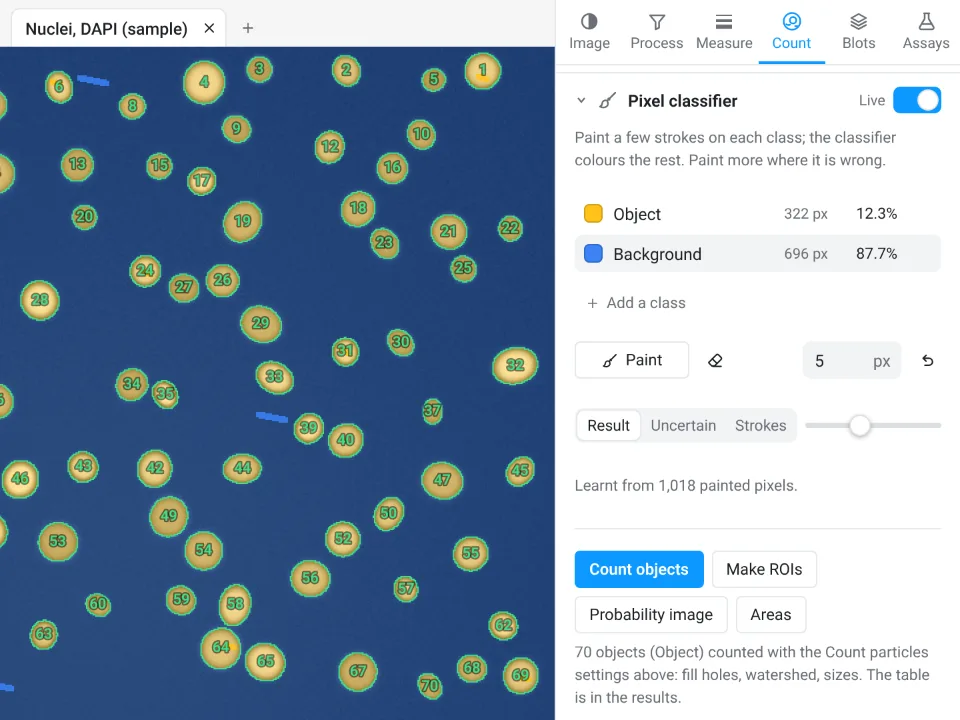
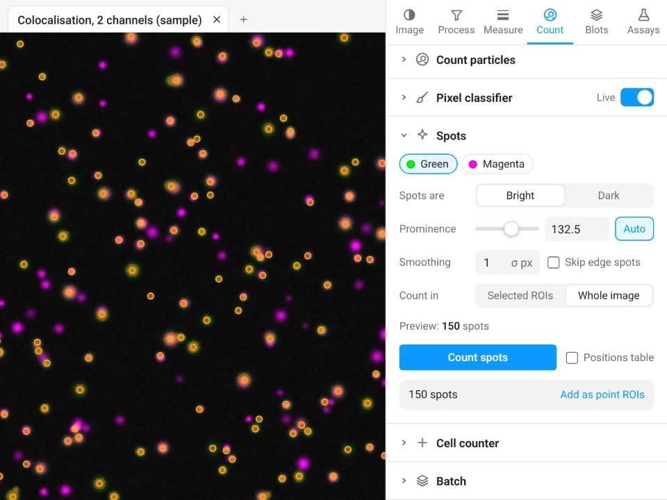
On the synthetic nuclei sample (70 nuclei by design), ImageJ counts 70 with Otsu, Fill Holes and Watershed, and Find nuclei in LabCanvas also counts all 70.
Why it is a good choice for cell counts:
- Nothing to install: it runs in the browser on any computer or tablet, so you can count at the bench.
- ImageJ's own names: Count particles is Analyze Particles, with the same sixteen threshold methods, fill holes, watershed, size and circularity.
- A pixel classifier built in, for cells a threshold cannot separate, instead of installing Trainable Weka Segmentation.
- An image check first: it flags clipped pixels, JPEG compression and uneven light (above 1.3×) before you count.
- Straight into Graphs: Send to Graphs plots the counts per condition, and every table carries a Methods sentence to copy. Counting, Copy and Send to Graphs are free with a LabCanvas account; downloading CSV files is part of LabCanvas Pro.
It does not run deep-learning segmentation (StarDist, Cellpose), 3D counting or macros, and files in a microscope maker's own format (.czi, .nd2, .lif) need exporting as TIFF first; for those, Fiji is the better tool. Every measurement is validated in more than 4,000 automated tests. Open Image Analysis. ImageJ and Fiji are independent open-source projects; LabCanvas is not affiliated with them.
References
- Arganda-Carreras I, Kaynig V, Rueden C, Eliceiri KW, Schindelin J, Cardona A, Seung HS (2017). Trainable Weka Segmentation: a machine learning tool for microscopy pixel classification. Bioinformatics 33, 2424–2426. doi:10.1093/bioinformatics/btx180
- Otsu N (1979). A threshold selection method from gray-level histograms. IEEE Transactions on Systems, Man, and Cybernetics 9, 62–66. doi:10.1109/TSMC.1979.4310076
- Schindelin J, Arganda-Carreras I, Frise E, et al. (2012). Fiji: an open-source platform for biological-image analysis. Nature Methods 9, 676–682. doi:10.1038/nmeth.2019
- Schneider CA, Rasband WS, Eliceiri KW (2012). NIH Image to ImageJ: 25 years of image analysis. Nature Methods 9, 671–675. doi:10.1038/nmeth.2089
- Stringer C, Wang T, Michaelos M, Pachitariu M (2021). Cellpose: a generalist algorithm for cellular segmentation. Nature Methods 18, 100–106. doi:10.1038/s41592-020-01018-x
Frequently asked questions
How do I count cells automatically in ImageJ?
Convert the image to 8-bit (Image › Type › 8-bit), set a threshold with Image › Adjust › Threshold so that the cells are red and the background is not, and click Apply. Then run Process › Binary › Fill Holes and Process › Binary › Watershed to split touching cells, and Analyze › Analyze Particles with a size range, Show: Outlines and Summarize ticked. The Summary window gives the count.
Where is the Cell Counter plugin in ImageJ?
Cell Counter comes with Fiji, under Plugins › Analyze › Cell Counter › Cell Counter: click Initialize, pick a counter type and click each cell, then Results for the counts. Plain ImageJ 1.x does not include it; there, use the Multi-point tool, whose options (double-click the tool) let you choose a counter for each class of cell.
How do I separate touching cells before counting?
Make a binary mask (threshold, then Process › Binary › Convert to Mask) and run Process › Binary › Watershed, which cuts touching round objects apart with one-pixel lines. It works well on nuclei, but it can cut long or irregular cells in two, so check the outlines. For crowded or irregular cells, deep-learning tools such as StarDist or Cellpose separate them better.
Why does Analyze Particles count only one huge particle?
The mask is the wrong way round: the background has become the object. Check Process › Binary › Options › Black background, make sure the cells are the thresholded (red) pixels before you apply the threshold, or invert the mask with Edit › Invert, and run Analyze Particles again.
Can ImageJ count cells in brightfield or phase-contrast images?
Not reliably with a plain threshold, because unstained cells differ from the background more in texture and halos than in brightness. A trained pixel classifier (Trainable Weka Segmentation in Fiji), a deep-learning tool such as Cellpose, or counting by hand works better. If you can, stain the nuclei and count those instead.
How do I convert a cell count to cells per mm²?
Divide the count by the area of the field in mm². The field area is the width times the height in pixels, times the pixel size squared: 512 × 512 pixels at 0.325 µm per pixel is 166.4 µm × 166.4 µm, or 0.0277 mm². For cells per mL from a hemocytometer, use the hemocytometer formula instead.
Is there an easier way to count cells without installing ImageJ?
Yes: LabCanvas Image Analysis runs in the browser and has Find nuclei, which thresholds, fills holes, splits touching nuclei and counts in one click; see the last section of this guide or open it at labcanvas.com/analysis.html.
Try it in LabCanvas
Every app is free to start in your browser. Create an account and begin.
Start Image Analysis free in your browserKeep reading
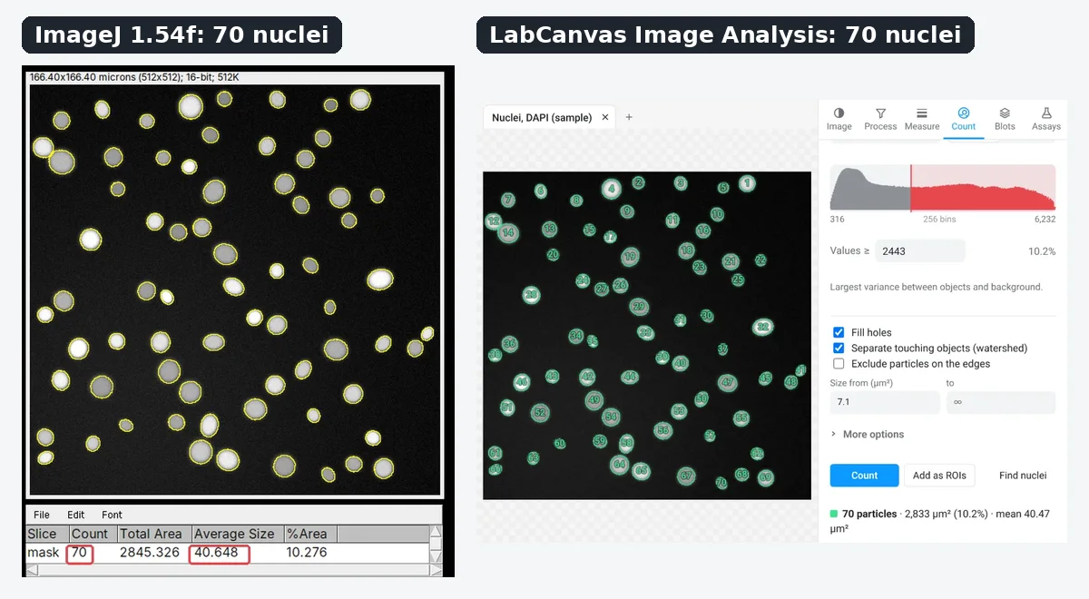
ImageJ vs LabCanvas Image Analysis: an honest comparison
ImageJ/Fiji or LabCanvas Image Analysis? Six everyday jobs done in both, six newer ones (macros, vendor files, 3D, StarDist, big images) and which to use.
How to use ImageJ: a beginner's tutorial for the 10 everyday jobs (2026)
How to use ImageJ and Fiji: get started, open an image, then 10 everyday jobs (scale, measure, threshold, count, background, blots) with exact menu paths.
How to set the scale and add a scale bar in ImageJ (with a calibration image to practise on)
Set the scale in ImageJ (Analyze › Set Scale) from a micrometer, scale bar or pixel size, add a scale bar, and practise on a free calibration image.