Image analysis guides
How to measure microscope images, electron micrographs, western blots and gels: set the scale, measure length and area, count cells and particles, quantify bands and fluorescence. Each guide gives the steps in ImageJ and Fiji, then the same job in LabCanvas Image Analysis, in your browser.
Start here
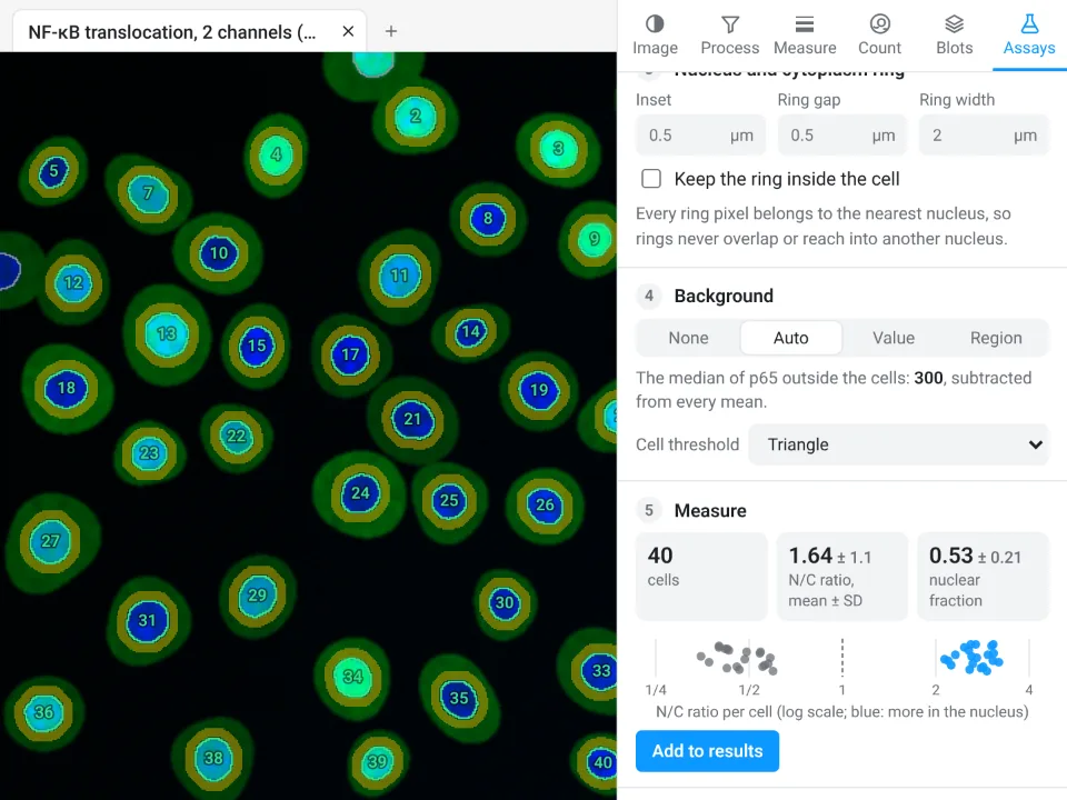
Image Analysis in LabCanvas: a complete guide to every tool and setting, with examples
Every tool in LabCanvas Image Analysis, tab by tab, with its settings and a real example: image check, display and scale, stacks and Z projection, background subtraction, filters, thresholds and binary operations, ROIs and Set measurements, Analyze Particles, a pixel classifier, spots, cell counter, western blot densitometry, colocalisation, colour deconvolution and eleven guided assays.
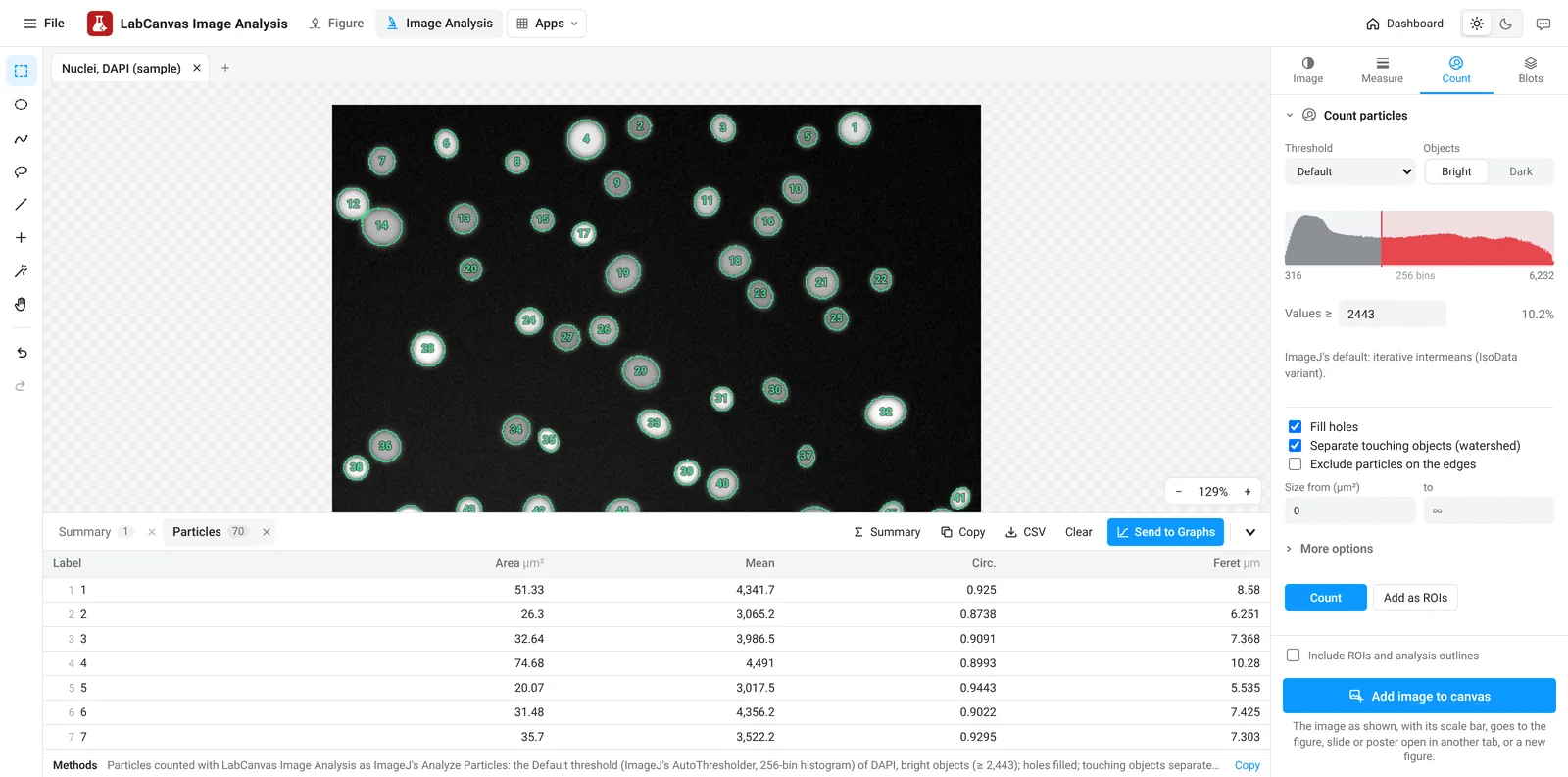
LabCanvas Image Analysis: measure microscopy images, western blots and gels in your browser
How to measure images in LabCanvas Image Analysis: guided assays (nuclear translocation, spots per cell, wound healing, FRAP, calcium, tracking, branching), western blots with a ladder and total-protein normalisation, cell counting with a trainable classifier, ROIs with ImageJ definitions, on the raw pixel values, with results sent to Graphs.
How-to guides
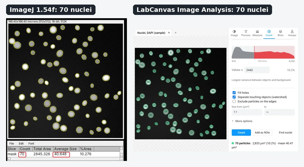
ImageJ vs LabCanvas Image Analysis: an honest comparison
ImageJ/Fiji or LabCanvas Image Analysis? Six everyday jobs done in both, six newer ones (macros, vendor files, 3D, StarDist, big images) and which to use.
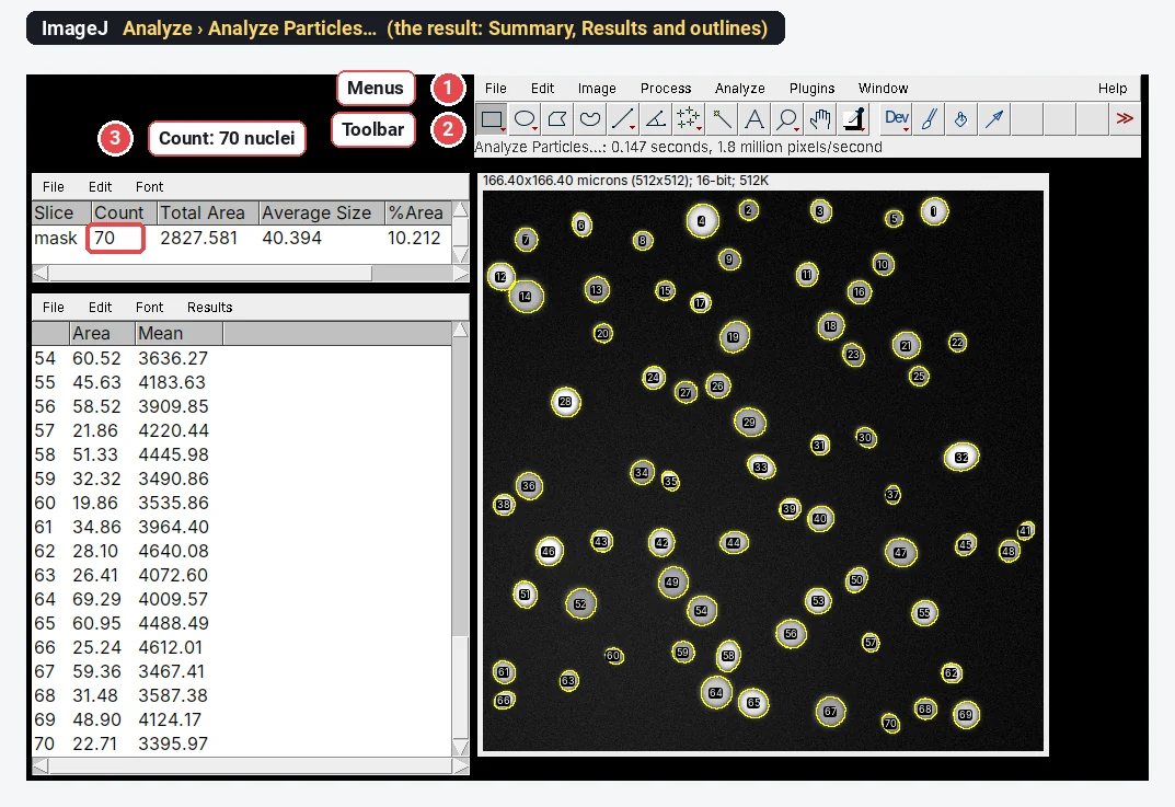
How to use ImageJ: a beginner's tutorial for the 10 everyday jobs (2026)
How to use ImageJ and Fiji: get started, open an image, then 10 everyday jobs (scale, measure, threshold, count, background, blots) with exact menu paths.
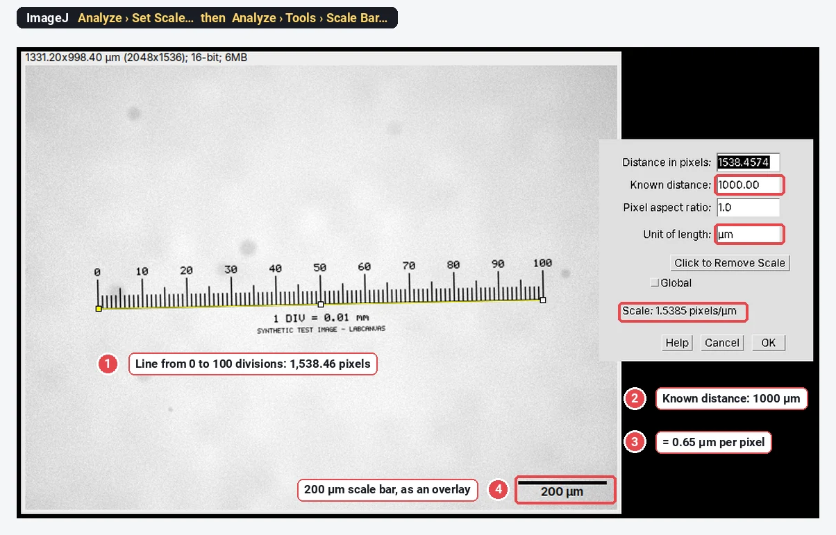
How to set the scale and add a scale bar in ImageJ (with a calibration image to practise on)
Set the scale in ImageJ (Analyze › Set Scale) from a micrometer, scale bar or pixel size, add a scale bar, and practise on a free calibration image.
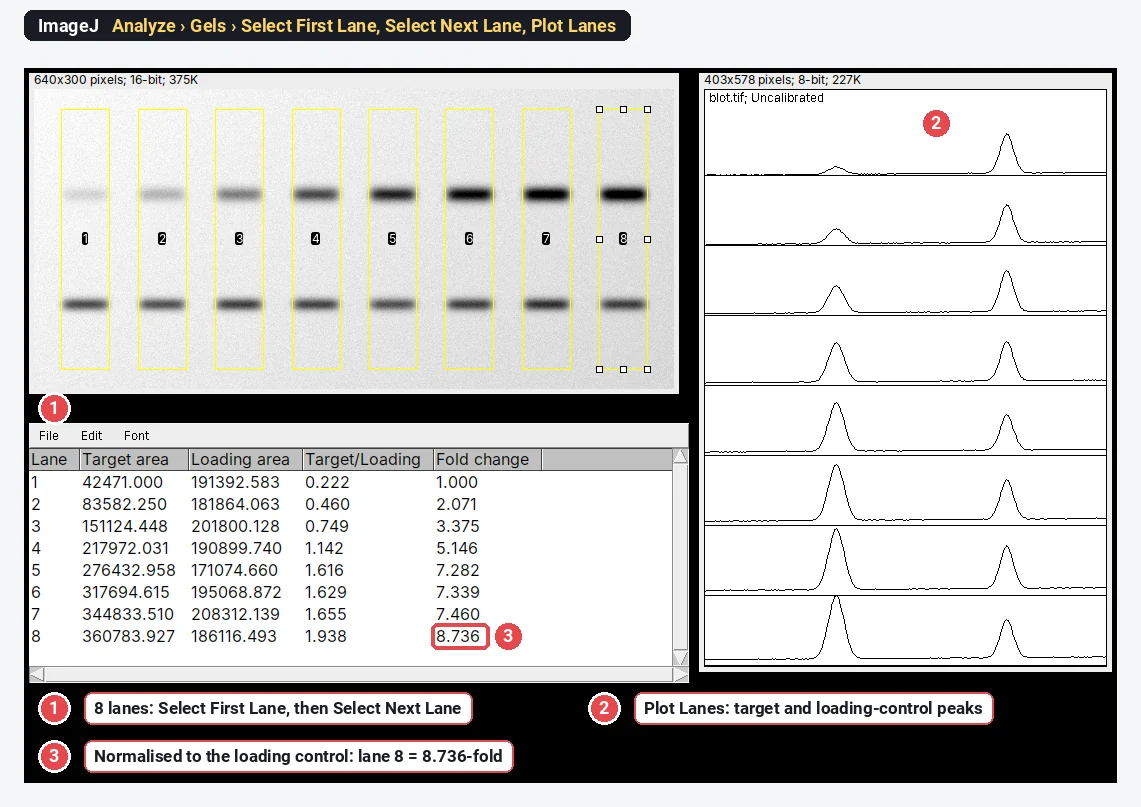
Western blot quantification in ImageJ, step by step (and the 3-click way)
Quantify a western blot in ImageJ with Analyze › Gels, normalise to a loading control or total protein, and get fold change. Plus a 3-click way.
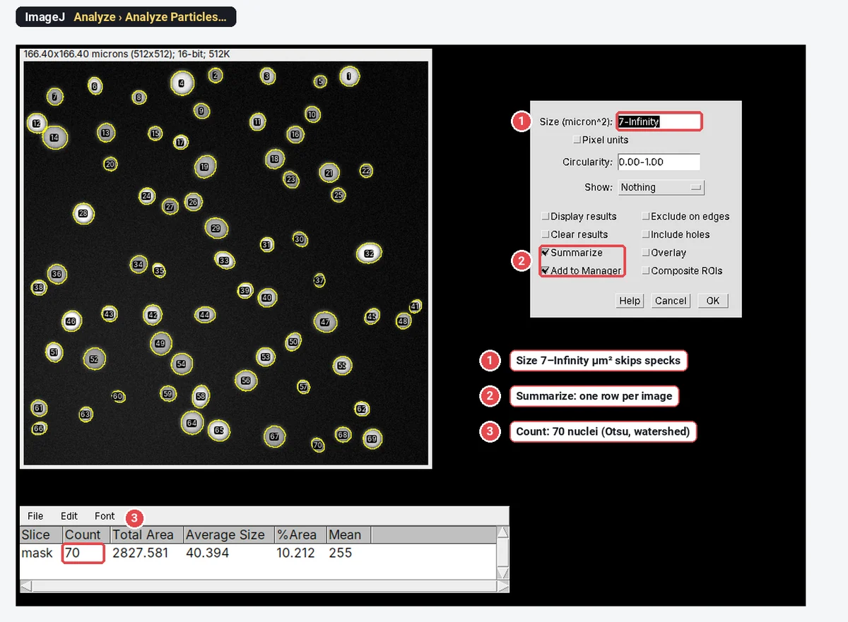
How to count cells in ImageJ (automatic and manual)
Count cells in ImageJ: automatic (threshold, Watershed, Analyze Particles) or manual (Cell Counter, Multi-point), plus cells per mm² and % positive.
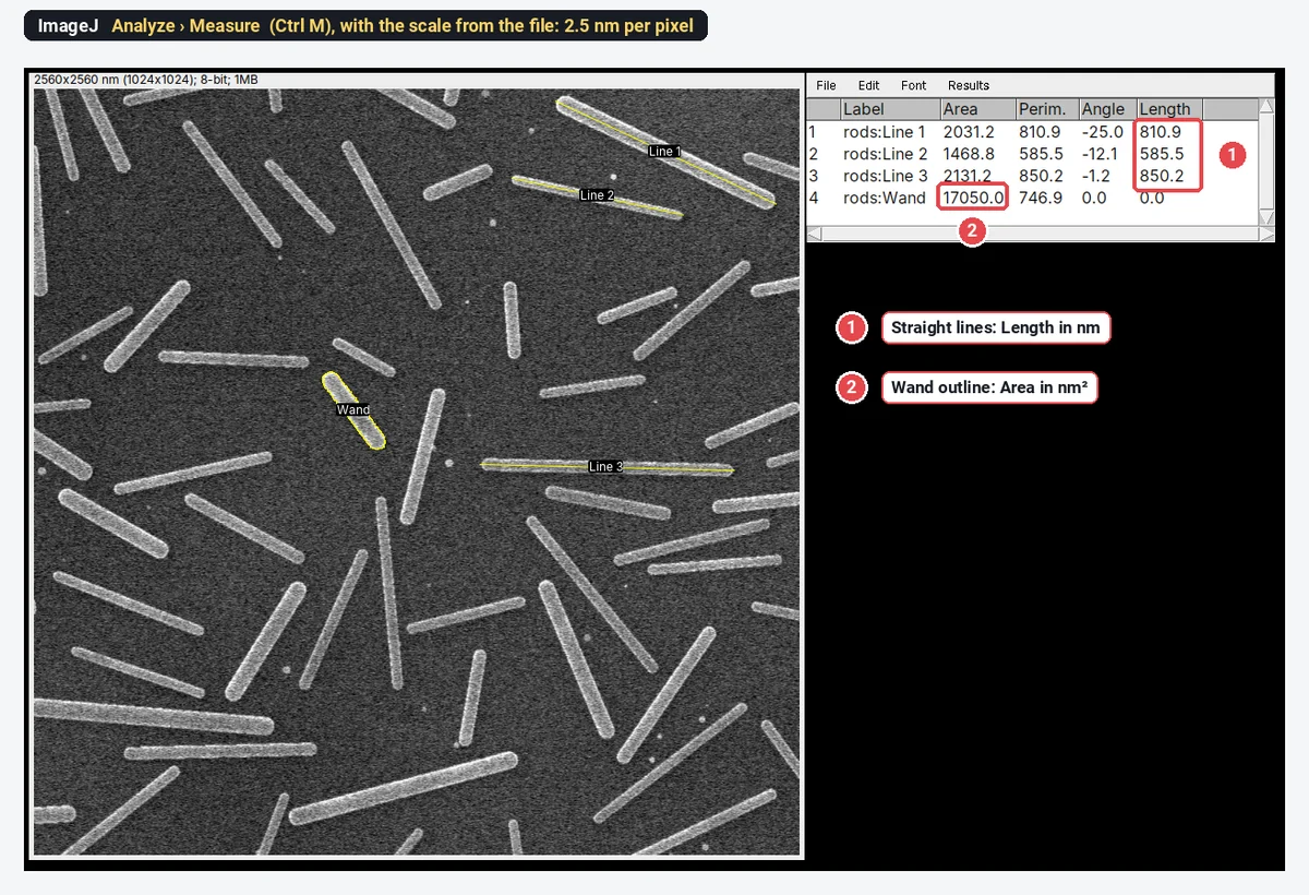
How to measure length and area in ImageJ (with the right units)
Measure length and area in ImageJ: set the scale, draw lines or area selections (polygon, wand, threshold), press Measure, and get µm and µm², not pixels.
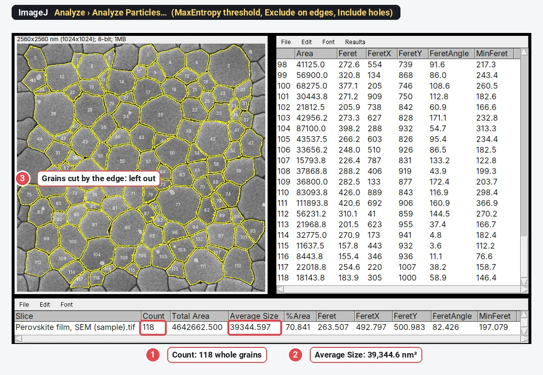
Grain size analysis in ImageJ (SEM, ASTM E112) + grain size number calculator
Measure grain size from SEM images in ImageJ: closed boundaries, Analyze Particles, then ASTM E112 G from mean area or intercept, with a worked example.
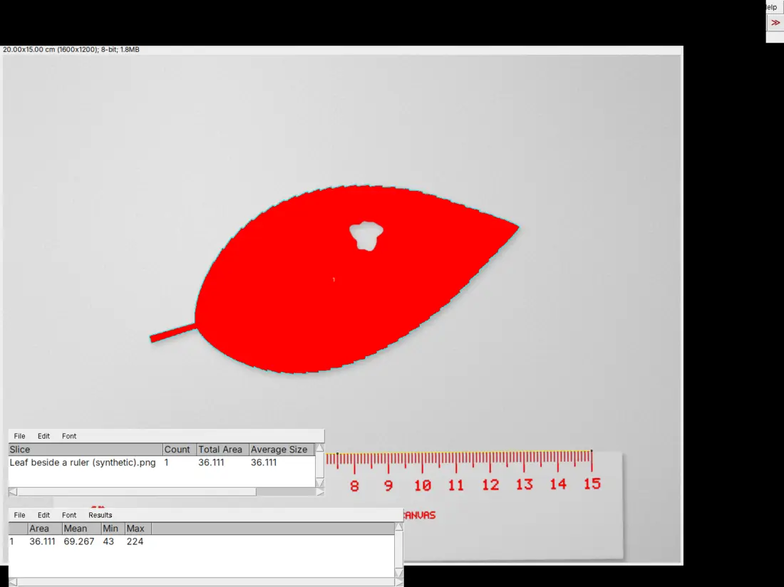
How to measure leaf area with ImageJ (or from a phone photo, in the browser)
Measure leaf area in ImageJ from a photo or scan: set the scale from a ruler, threshold the leaf, run Analyze Particles in cm², with or without holes.
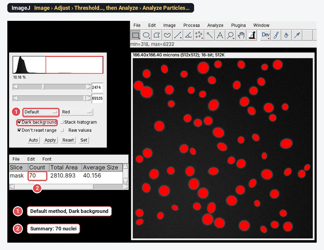
ImageJ online: can you run it in a browser? (ImageJ.JS, and a faster way)
Yes: ImageJ.JS runs ImageJ 1.x in your browser via CheerpJ (WebAssembly). What works, what doesn't, Fiji online, iPad and Android, and a faster option.
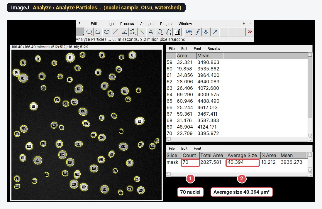
Best ImageJ alternatives in 2026 (free, online and desktop)
The best ImageJ alternatives compared: browser tools, Fiji, CellProfiler, QuPath, ilastik, napari, Icy, MIPAR, and Image Lab and Empiria for blots.
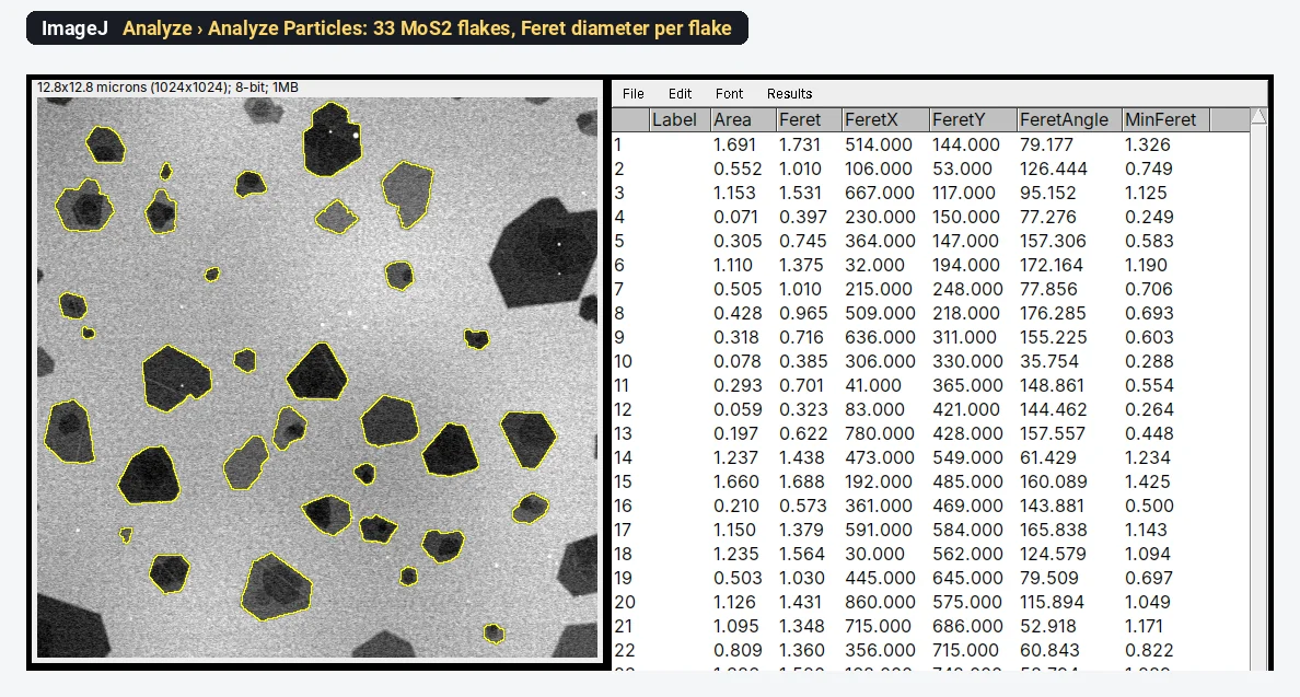
Lateral size of 2D flakes (graphene, MoS₂) from SEM or TEM in ImageJ
Measure graphene or MoS₂ flake lateral size in ImageJ: scale, threshold, Analyze Particles with Feret diameter, edge flakes, overlaps and a size histogram.
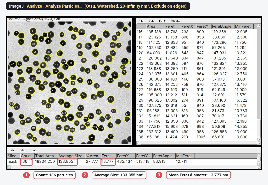
Analyze Particles in ImageJ, explained (every option, with examples)
Every Analyze Particles option in ImageJ, shown on a TEM image: size, circularity, Show, Exclude on edges, Include holes, and why it finds 0 or 1 particle.
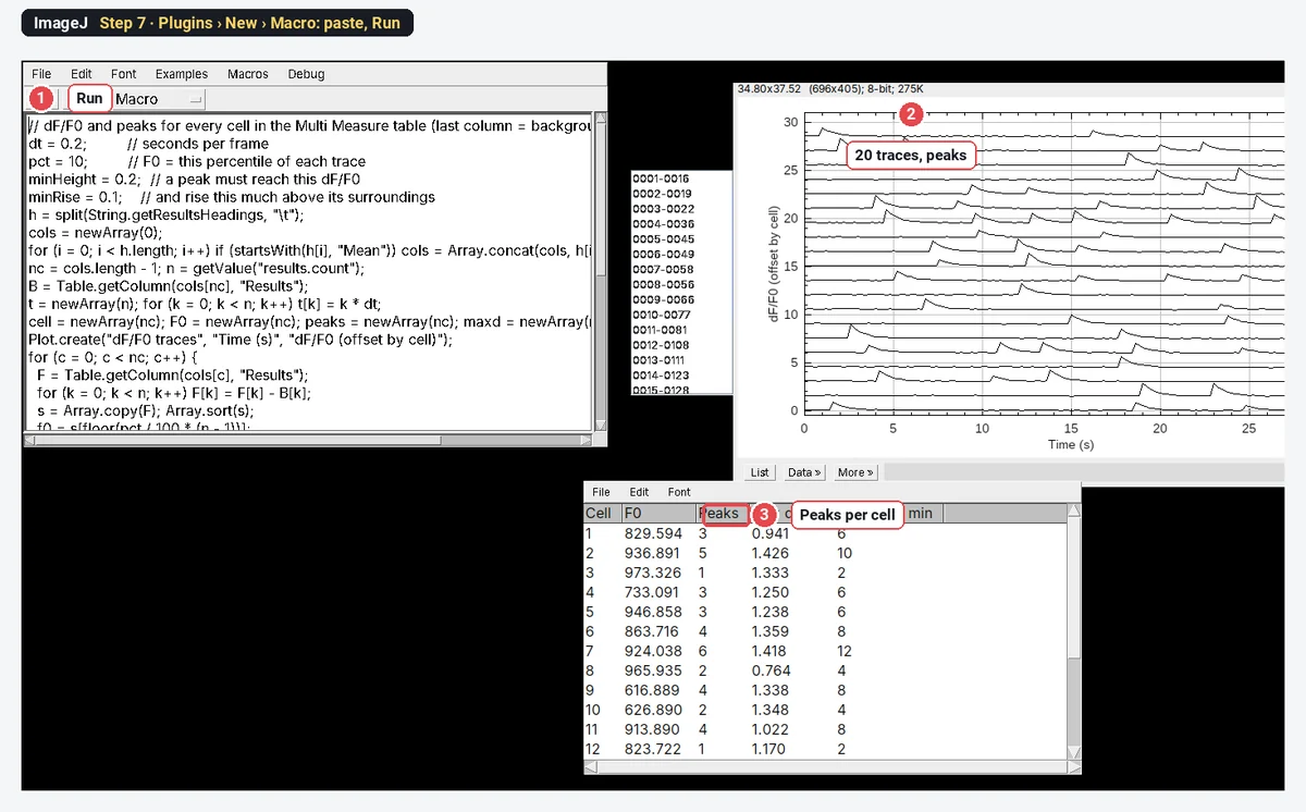
Calcium imaging analysis in ImageJ: ΔF/F₀ traces step by step
Calcium imaging in ImageJ: ROIs on cells, Multi Measure, background, F₀ (first frames or a percentile), ΔF/F₀ = (F − F₀)/F₀, traces and peak counting.
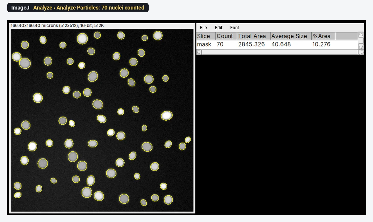
CellProfiler vs QuPath vs ImageJ: which image analysis software should you use?
CellProfiler, QuPath or ImageJ/Fiji? A fair comparison by job (batch cell measurements, whole slides, general analysis), with a nuclei count step by step.
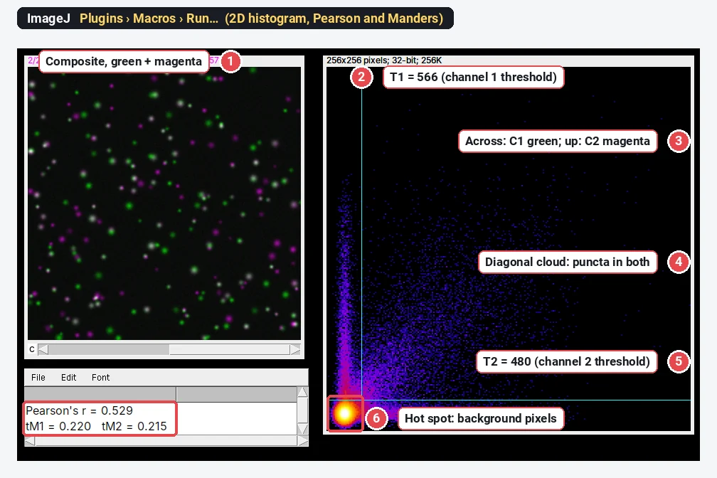
Colocalization analysis in ImageJ: Pearson vs Manders and Costes thresholds
Colocalization in ImageJ and Fiji: what Pearson’s r and Manders’ M1/M2 each answer, Costes thresholds, Coloc 2 vs JACoP, a worked example and pitfalls.
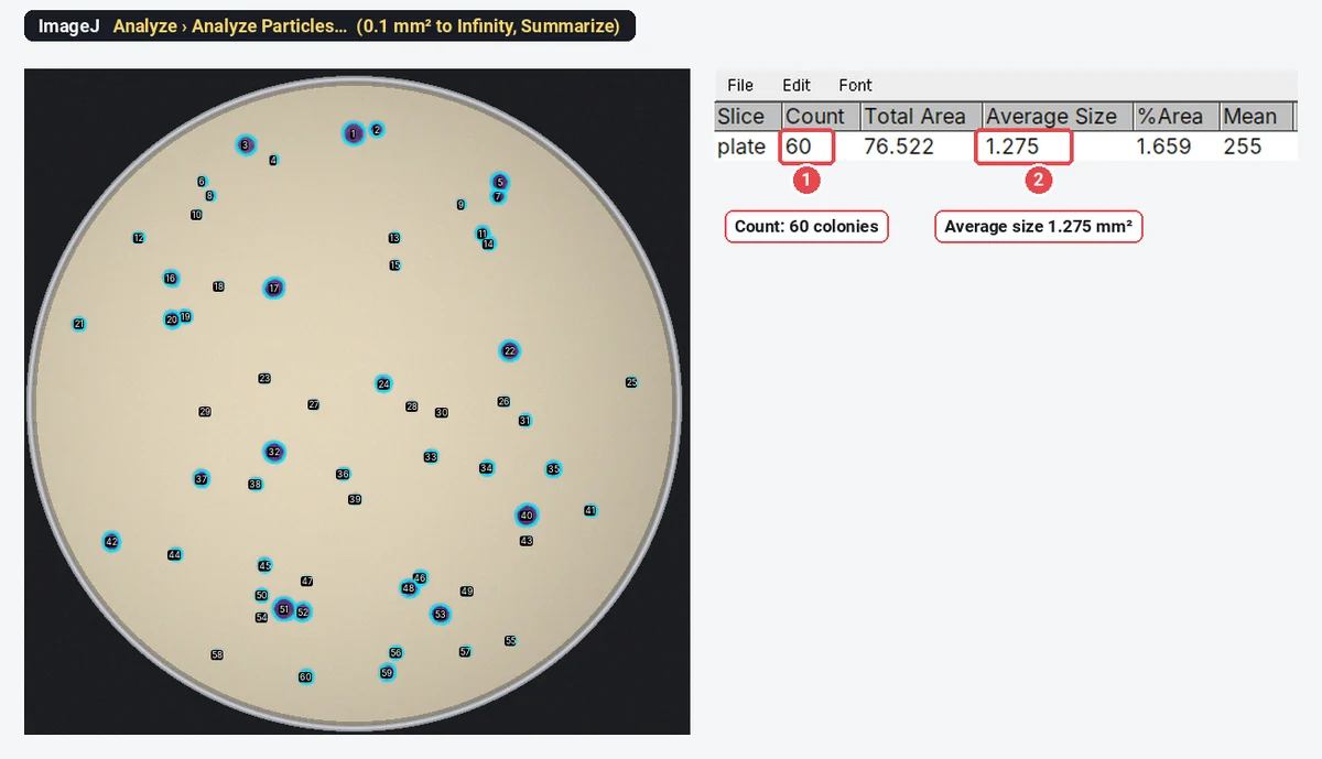
Count bacterial colonies in ImageJ (or from a plate photo, free online)
Count colonies in ImageJ: oval on the dish, threshold, Watershed, Analyze Particles. Then CFU/mL from the count and dilution, with a worked example.
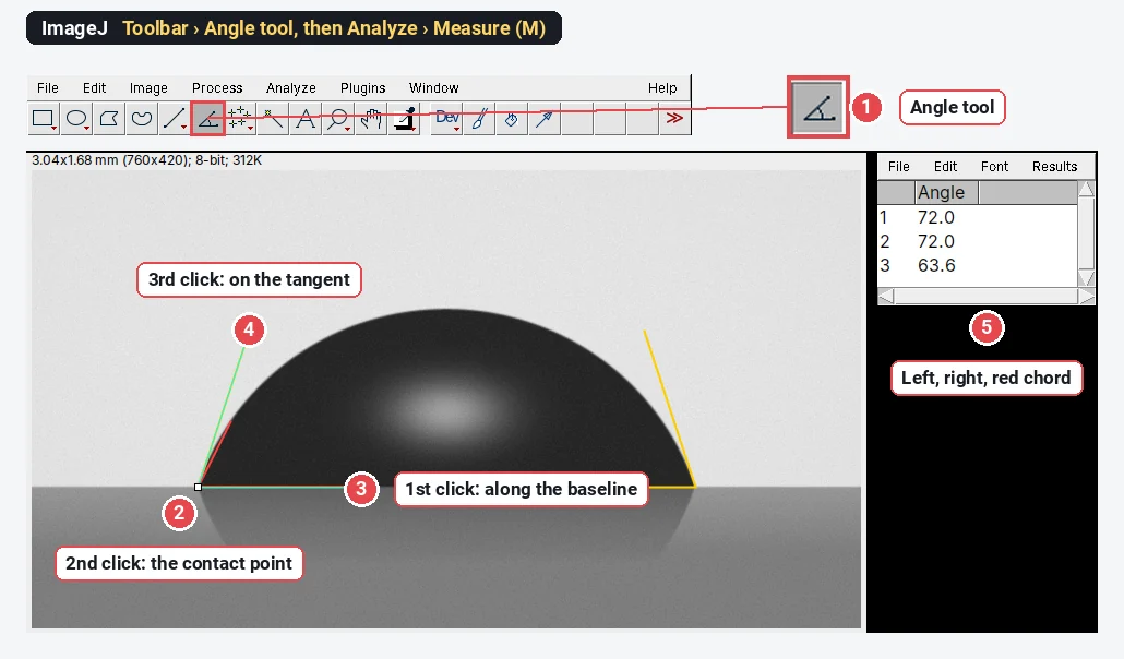
Measure contact angle from a drop photo in ImageJ
Measure contact angle in ImageJ with the Angle tool along the tangent, or from drop height and base width: θ = 2·arctan(2h/d). Worked example, plugins.
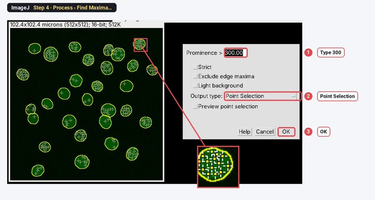
Count γH2AX or 53BP1 foci per nucleus in ImageJ (Find Maxima, step by step)
Count γH2AX or 53BP1 foci per nucleus in ImageJ: nuclei as ROIs, Find Maxima with the right prominence, counts per nucleus and % of cells with ≥5 foci.
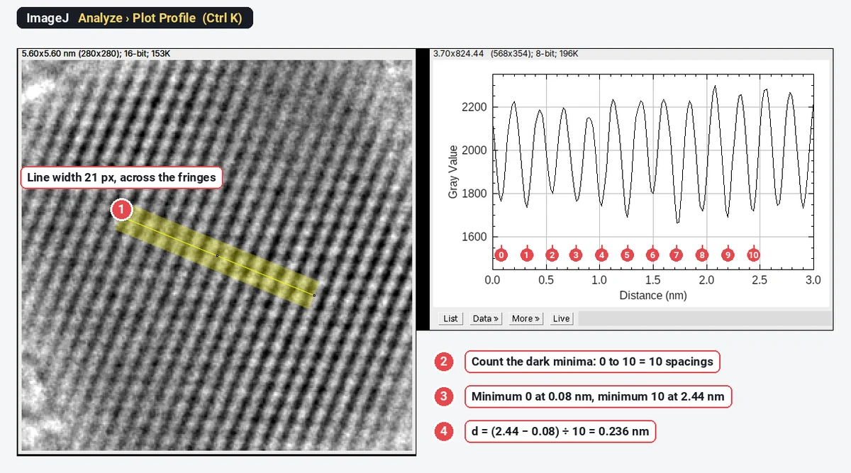
How to measure d-spacing from HRTEM lattice fringes in ImageJ (profile and FFT)
Measure d-spacing in ImageJ: a wide line across 10 fringes and Plot Profile (d = L ÷ N), or FFT spots read with Measure. Worked on Au (111), 0.235 nm.
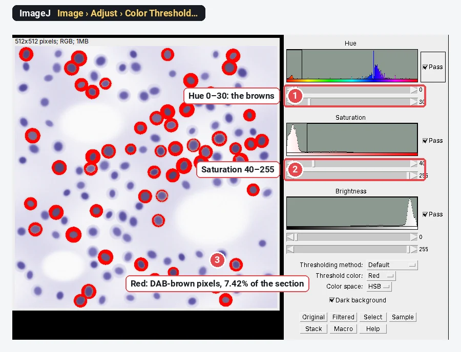
IHC DAB quantification in ImageJ with colour deconvolution
Quantify DAB IHC in ImageJ/Fiji: colour deconvolution with H-DAB vectors, % positive area, optical density, and why DAB intensity is not linear.
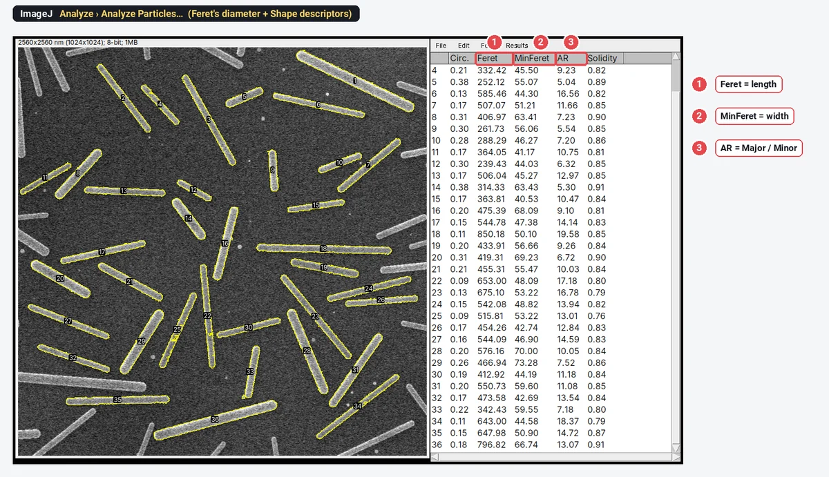
Feret diameter, circularity, aspect ratio and solidity in ImageJ, explained
What ImageJ shape descriptors mean: Feret and MinFeret, circularity, AR, roundness and solidity, with formulas, drawn shapes and real TEM and SEM numbers.
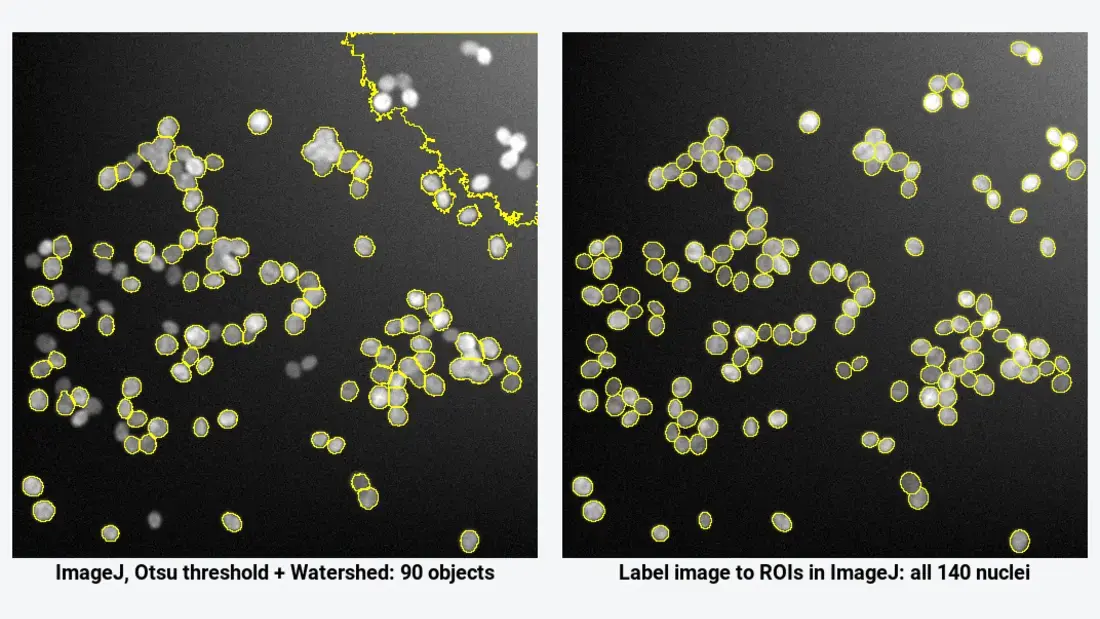
Deep-learning cell segmentation in Fiji: StarDist, Cellpose and Weka (step by step)
When a threshold fails, segment cells in Fiji with StarDist, Cellpose or Trainable Weka: install, settings, then label image to ROIs and measurements.
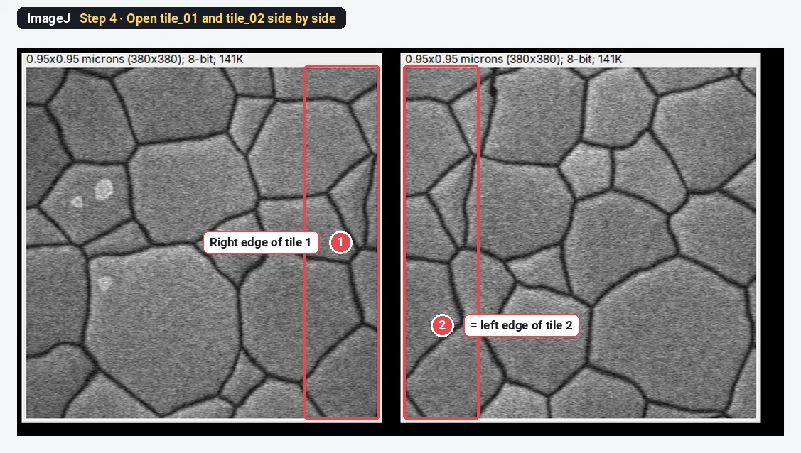
Stitch microscope tiles in Fiji (Grid/Collection stitching, step by step)
Stitch overlapping microscope tiles in Fiji with Grid/Collection stitching: grid type, overlap, file names, fusion, and why an ImageJ montage is wrong.
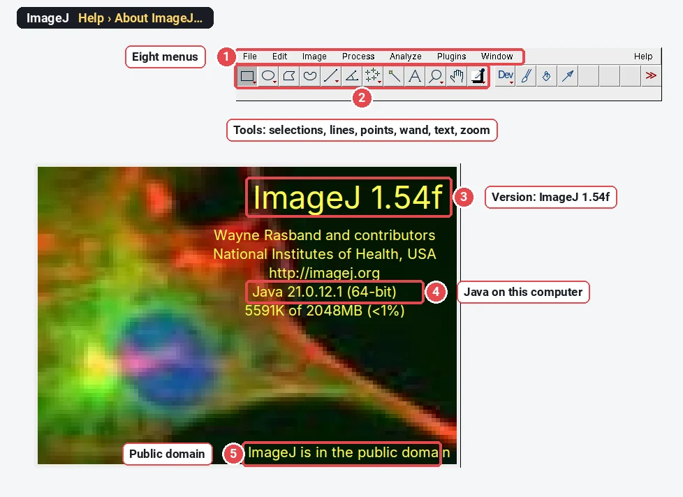
Fiji vs ImageJ: what's the difference, and which should you download?
Fiji is ImageJ with plugins, Bio-Formats, an updater and scripting built in; ImageJ2 is the rewrite underneath. A comparison table and which to download.
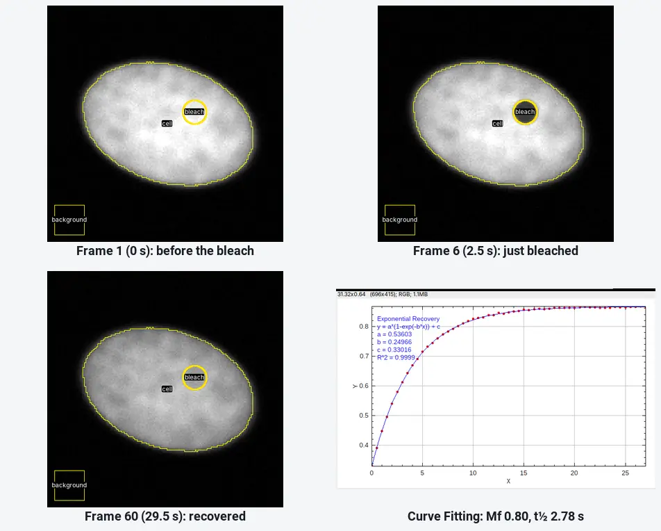
FRAP analysis in ImageJ: mobile fraction and half-time, step by step
FRAP in ImageJ: bleach, reference and background ROIs, Multi Measure, double normalisation, an exponential recovery fit, then the mobile fraction and t½.
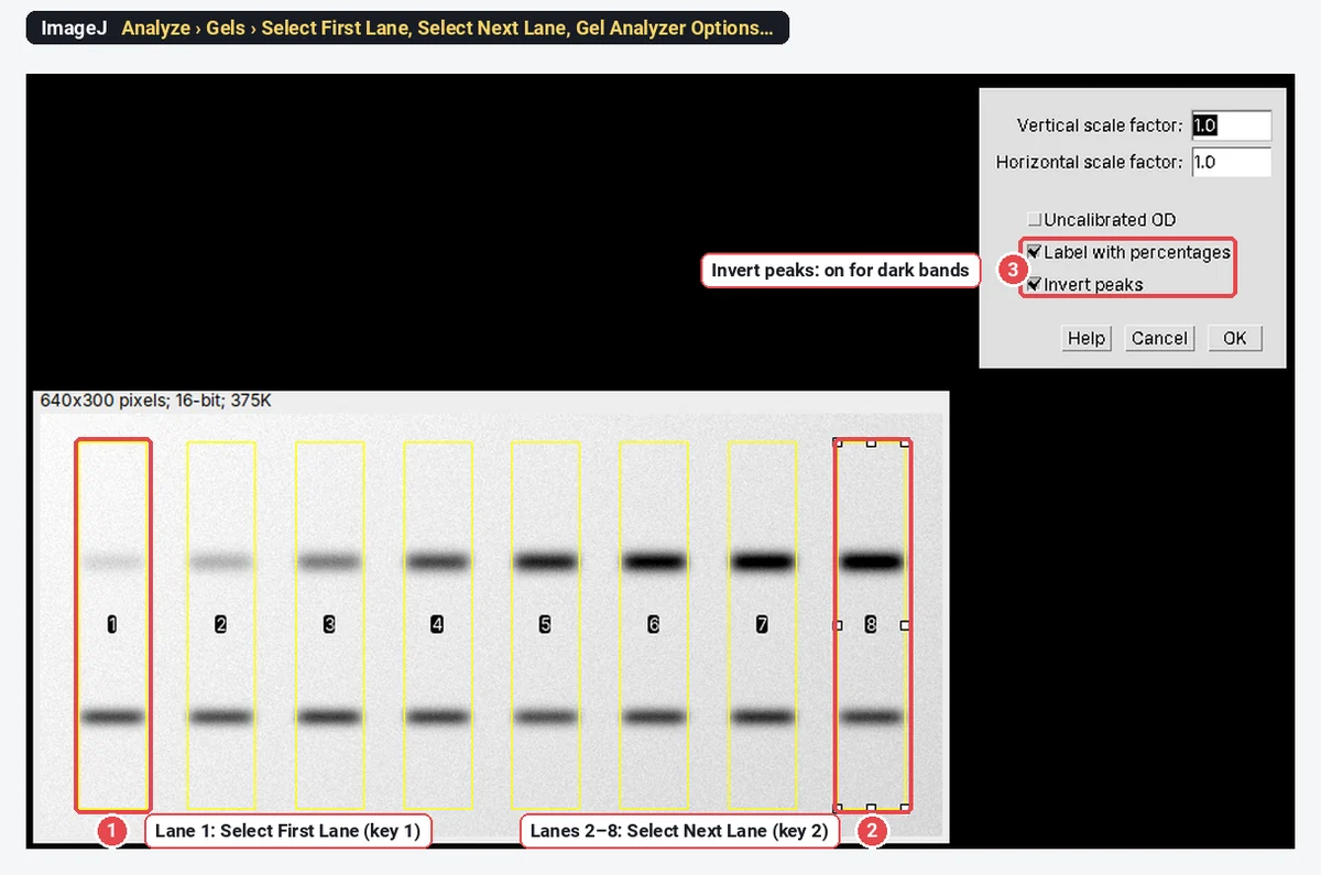
Free western blot quantification software (now that Image Studio Lite is gone)
Image Studio Lite is discontinued. Quantify western blots free in ImageJ (Analyze › Gels), step by step, with Image Lab and IOCBIO Gel compared.
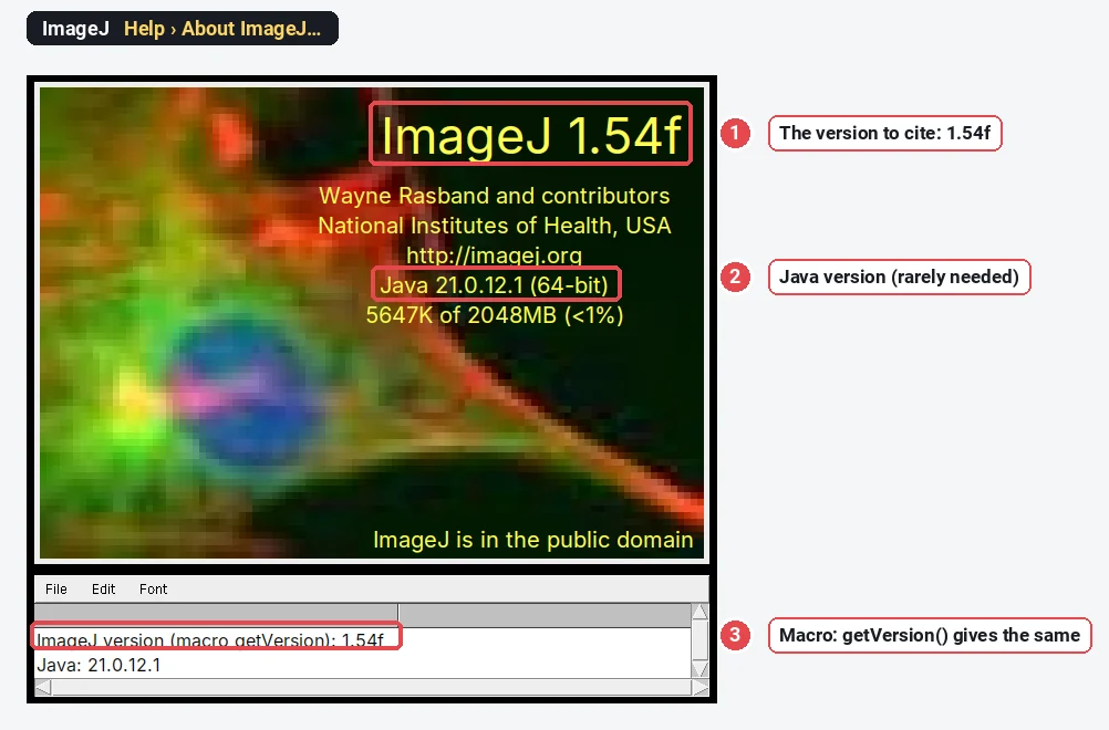
How to cite ImageJ and Fiji (with a methods sentence to copy)
Cite ImageJ (Schneider et al. 2012), Fiji (Schindelin et al. 2012) or ImageJ2 (Rueden et al. 2017): DOIs, APA, Vancouver, BibTeX and methods sentences.
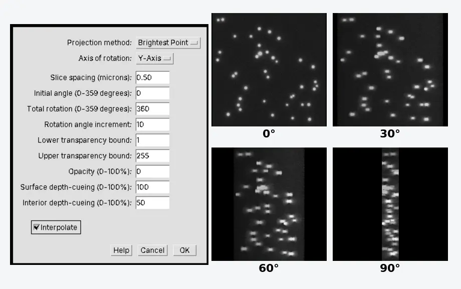
3D projection and 3D viewing in ImageJ (Image › Stacks › 3D Project)
Make a rotating 3D view of a Z-stack with Image › Stacks › 3D Project in ImageJ, set the slice spacing, use Orthogonal Views, or Fiji's 3D Viewer.
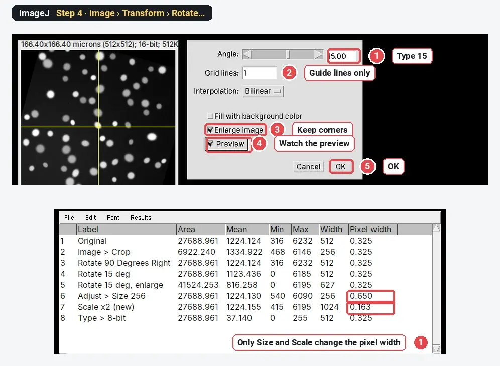
Crop, rotate, resize and convert images in ImageJ (without changing your data by accident)
How to crop, rotate, resize, zoom and convert to 8-bit or grayscale in ImageJ, and what each command does to pixel values and the scale, measured.
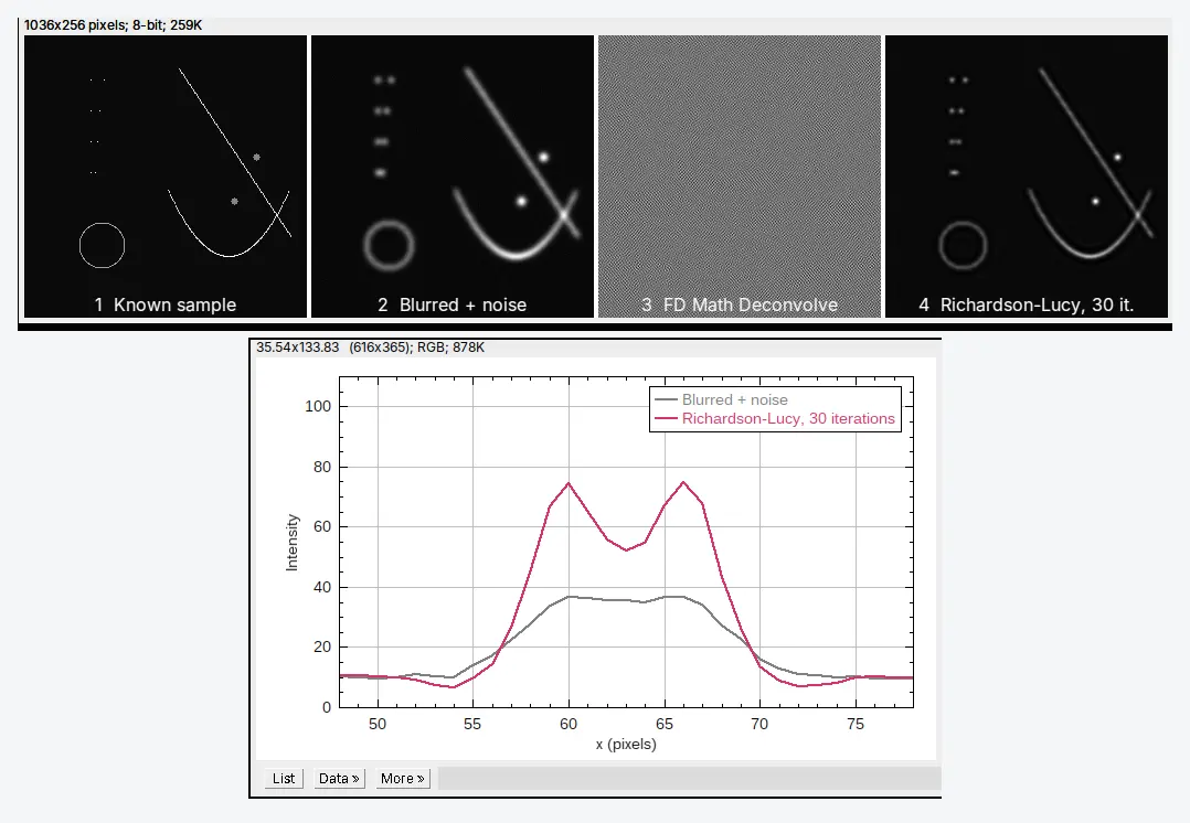
Deconvolution in ImageJ and Fiji: what it does and how to run it
What deconvolution does (the PSF, Richardson–Lucy), why FD Math Deconvolve fails on real images, and how to run Richardson–Lucy in ImageJ and Fiji.
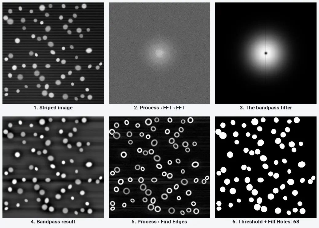
FFT bandpass filter and edge detection in ImageJ (with before/after examples)
FFT in ImageJ step by step: Process › FFT, Bandpass Filter settings, stripe removal and Find Edges, with before/after pictures and when filtering is safe.
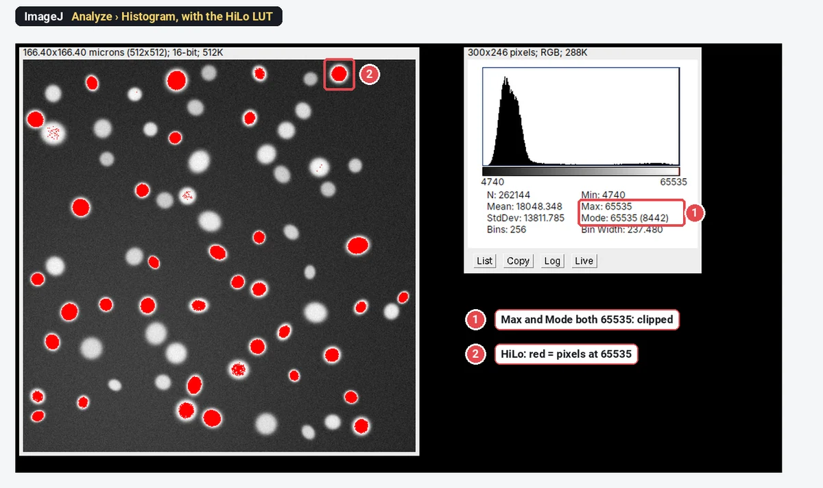
Check for saturated pixels in ImageJ: histogram, HiLo LUT and the numbers
Check saturation in ImageJ with Analyze › Histogram, the HiLo LUT and Min/Max, on a clipped example with its spike at 65535 and what it does to data.
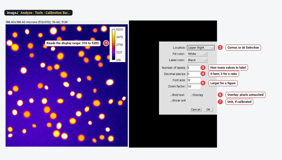
LUTs in ImageJ: which lookup table to use (and colour-blind-safe choices)
ImageJ lookup tables compared on one image: Grays, Fire, viridis, HiLo and the rest, how to add a calibration bar, and colour-blind-safe channel colours.
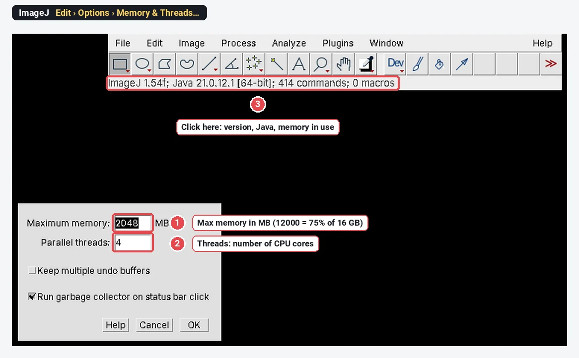
ImageJ and Fiji on a Mac: install, Apple Silicon and "can't be opened" fixes
Download ImageJ or Fiji for Mac (Apple Silicon or Intel), fix "can't be opened" and "damaged" errors, set the memory, and the no-install option.
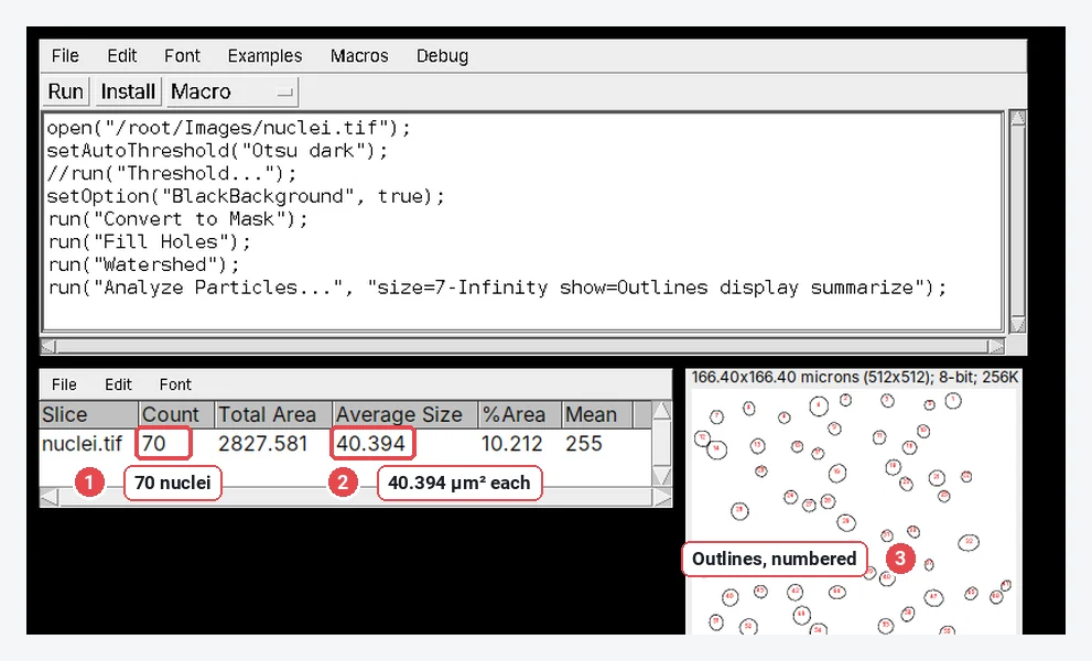
ImageJ macros for beginners: record a macro and batch-process a folder
Record an ImageJ macro with Plugins › Macros › Record, run it from the editor, then batch-process a folder with Process › Batch › Macro. Step by step.
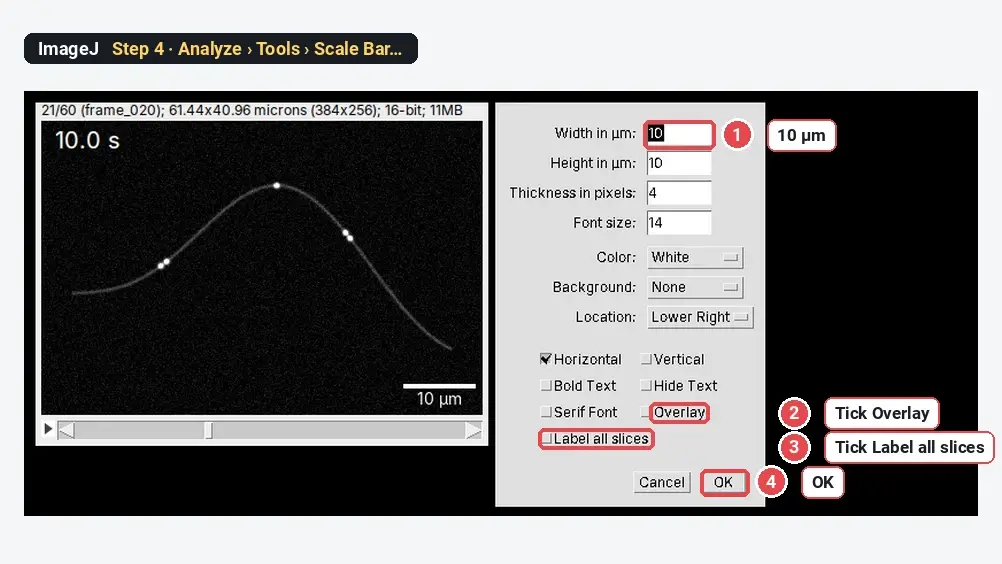
Make a movie from an image stack or time-lapse in ImageJ (AVI, GIF, MP4)
Turn a folder of frames or a time-lapse stack into an AVI, GIF or MP4 in ImageJ: Image Sequence, a time stamp, a scale bar, frame rate, and saving.
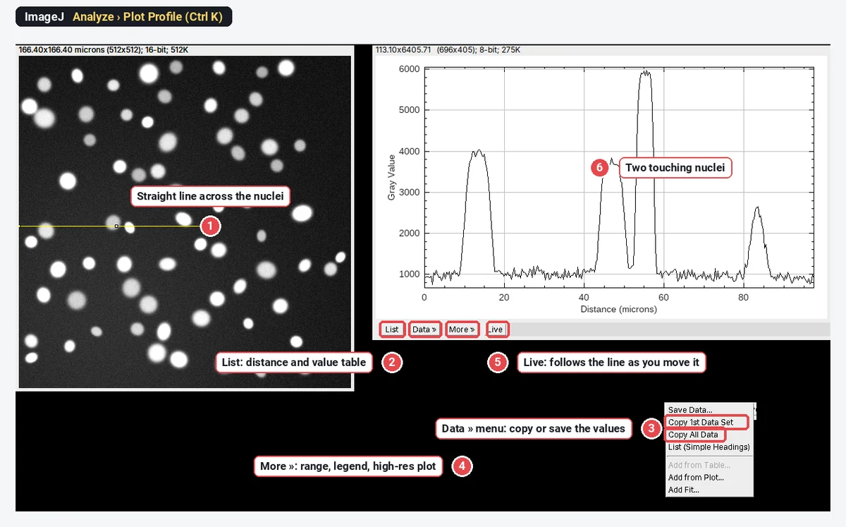
Plot Profile in ImageJ: line scans, wide lines and intensity profiles
Plot Profile in ImageJ: draw a line, press Ctrl K, set the line width to average noise, copy the values, plot two channels and profile a rectangle.
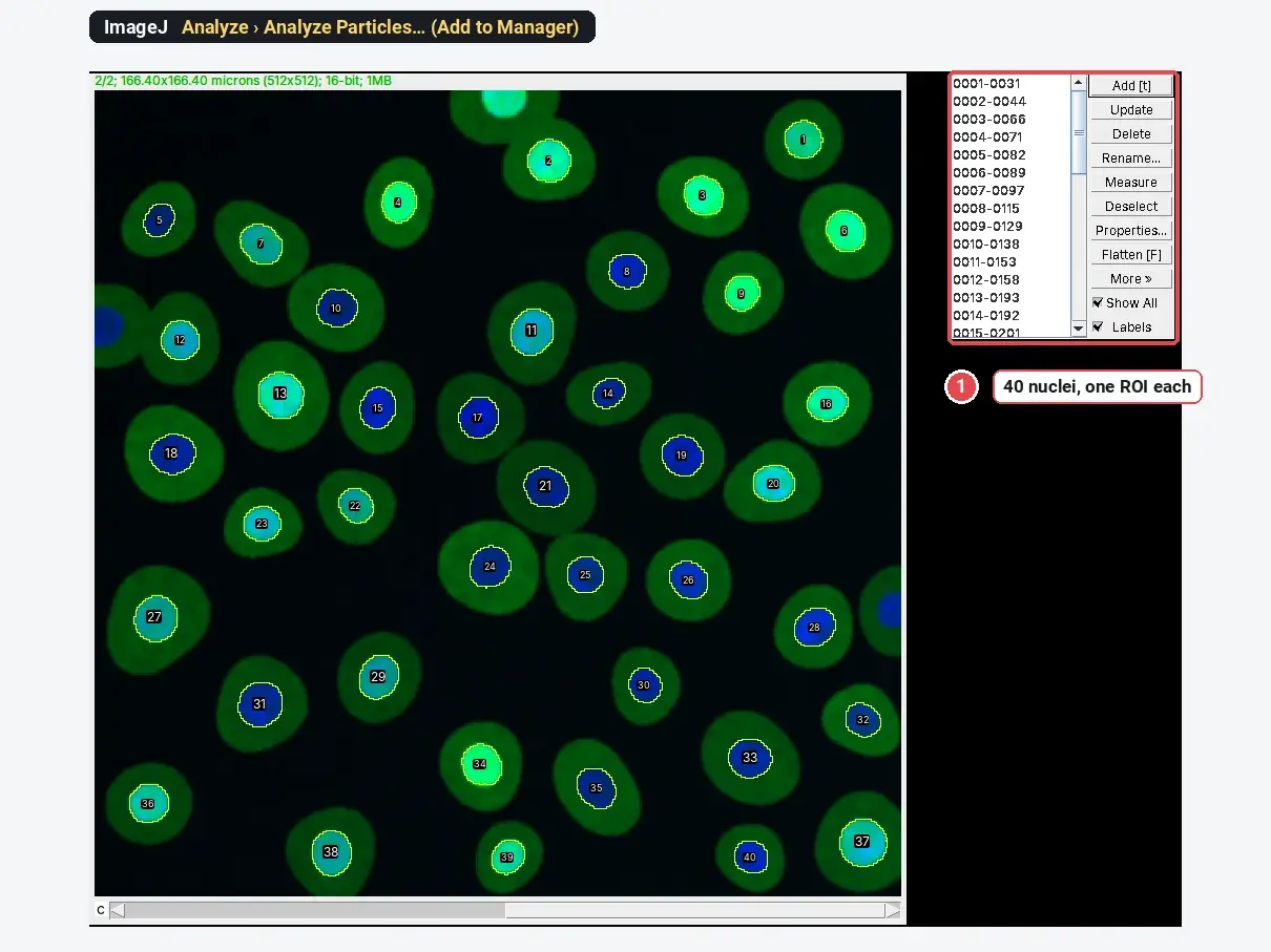
ROI Manager in ImageJ: measure many regions, save them and open them anywhere
Open the ROI Manager in ImageJ (Analyze › Tools › ROI Manager), add ROIs with T, measure them on every channel, save RoiSet.zip and reopen it later.
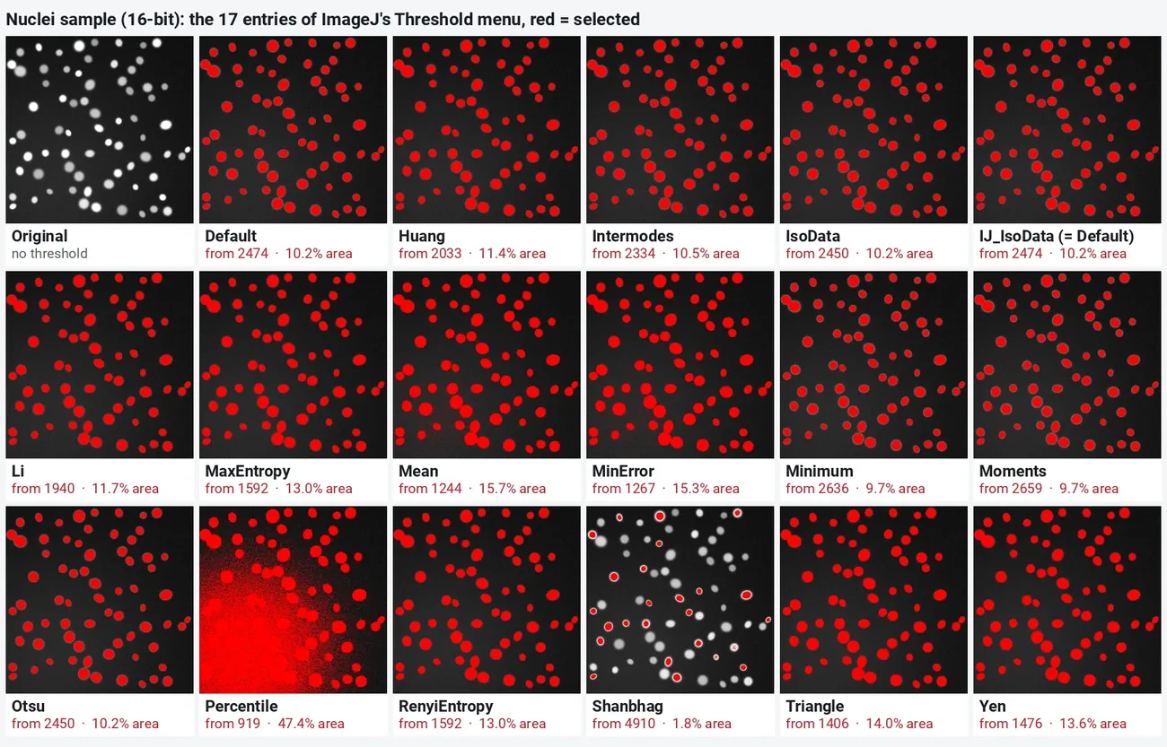
ImageJ threshold methods compared, with pictures
All 16 ImageJ auto threshold methods on one image, with the threshold and % area each gives, which method suits which image, and how to apply it.
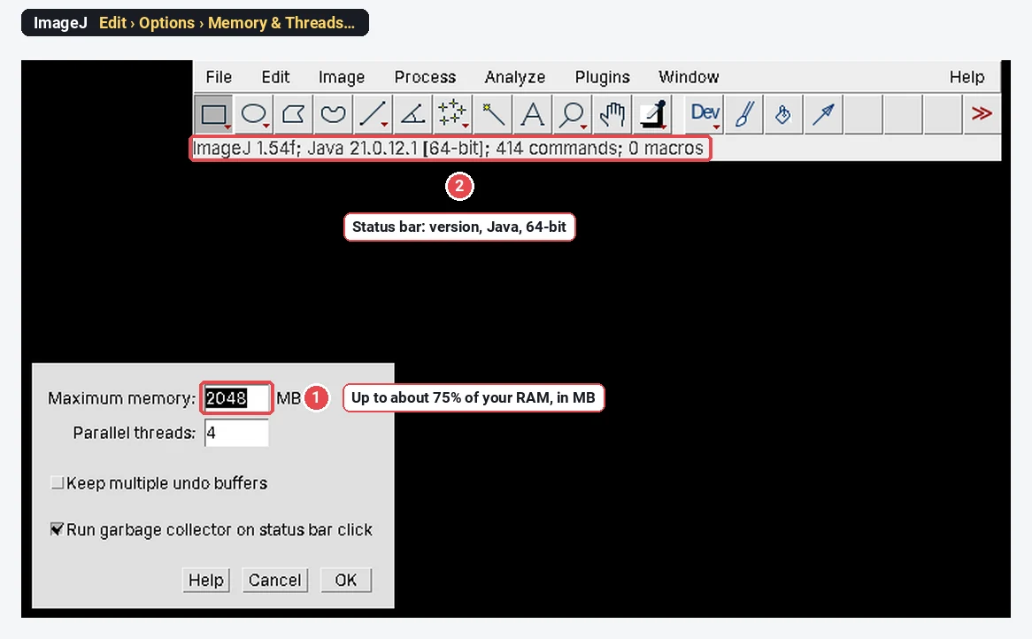
Install ImageJ or Fiji on Windows 10 and 11
Download and install Fiji or ImageJ on Windows 10 and 11: the right zip, where to unzip it (not Program Files), Java, memory, and where files go.
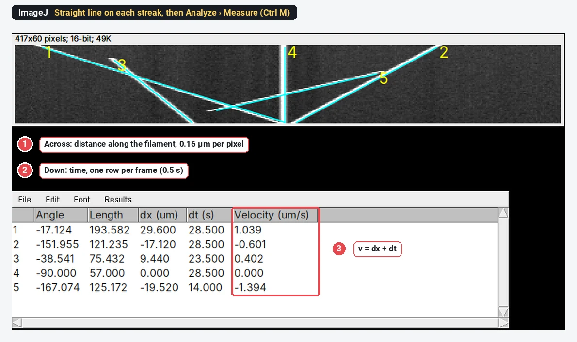
How to make a kymograph in ImageJ and measure velocities
Make a kymograph in ImageJ: a line along the track, Image › Stacks › Reslice, then a line on each streak gives velocity = Δx ÷ Δt, with a worked example.
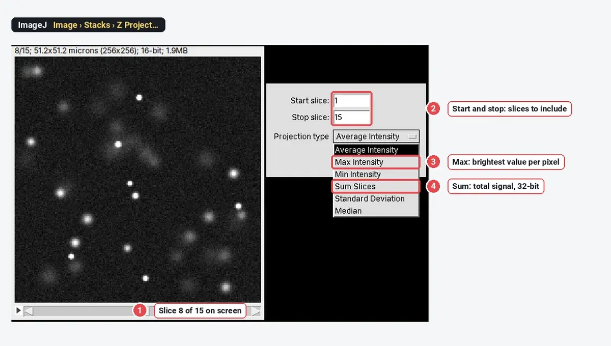
Z Project in ImageJ: maximum, average and sum projections compared
Image › Stacks › Z Project in ImageJ: what Max Intensity, Average, Sum Slices, SD, Min and Median give, when Sum beats Max, and how to check depth.
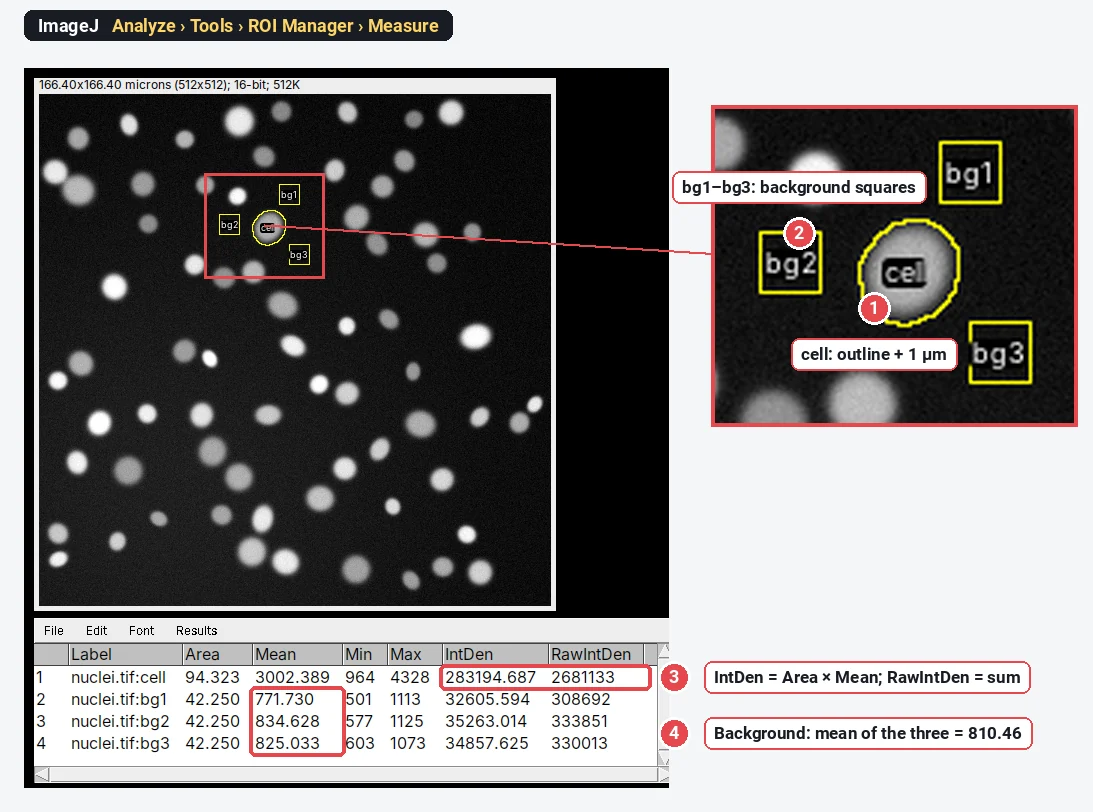
How to measure fluorescence intensity in ImageJ (Mean, IntDen, RawIntDen and CTCF)
Measure fluorescence in ImageJ: Mean, IntDen and RawIntDen explained, CTCF = IntDen − Area × background worked through, and the 8-bit and saturation traps.
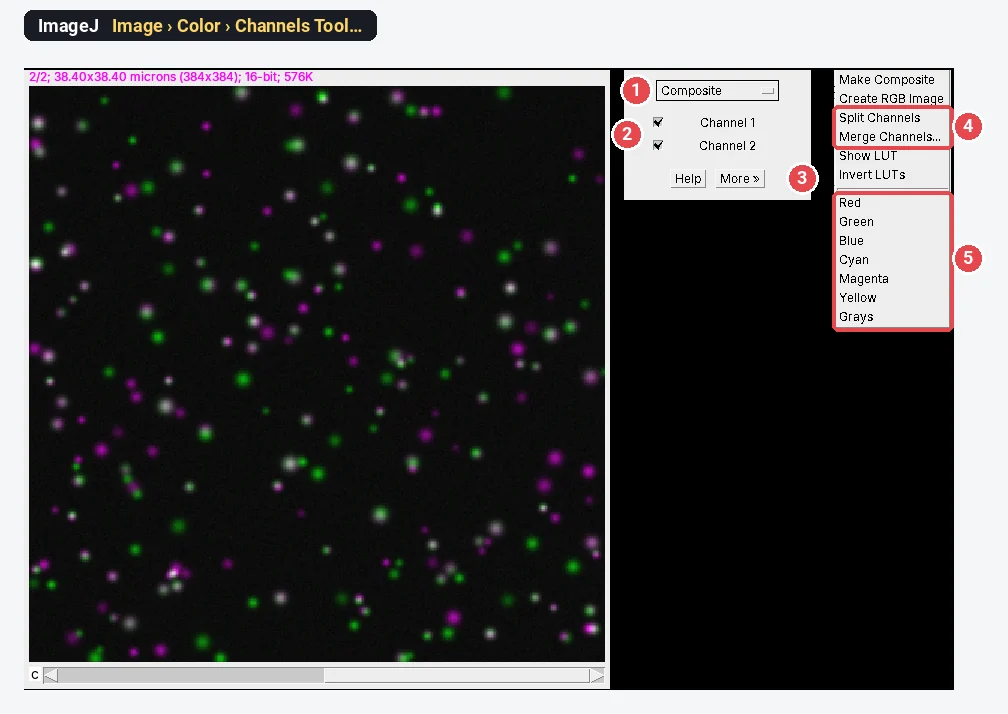
Merge, split and overlay channels in ImageJ (and make a composite figure)
Merge channels in ImageJ with Image › Color › Merge Channels, split them with Split Channels, overlay with Add Image, and build a colour-blind-safe figure.
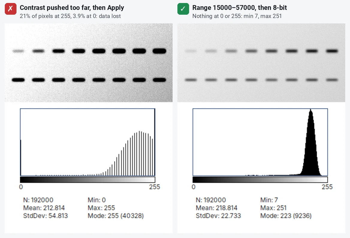
Image integrity: what you may and may not do to microscopy and blot images
What journals allow when you adjust microscopy and blot images: linear whole-image changes, gamma disclosed, no cloning or selective edits, in ImageJ.
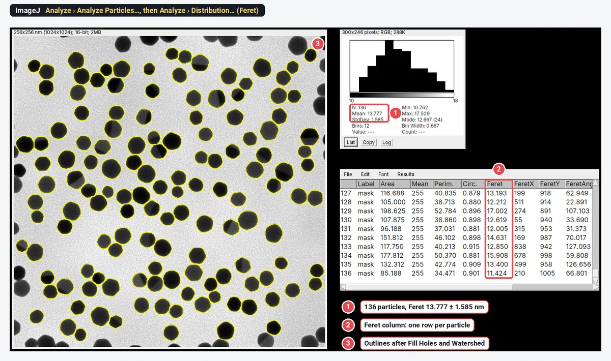
Nanoparticle size distribution from TEM images in ImageJ (step by step)
Nanoparticle size from TEM in ImageJ: scale, threshold, watershed, Analyze Particles with Feret, then the size histogram and mean ± SD, worked through.
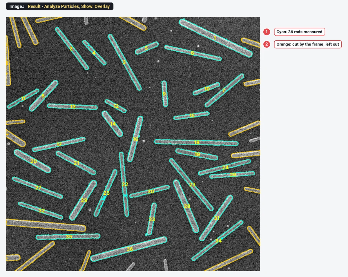
Nanorod and nanowire length, width and aspect ratio from SEM images in ImageJ
Measure nanorod and nanowire length, width and aspect ratio from SEM images in ImageJ: Feret, MinFeret, fit ellipse, edge rods, and why not to watershed.
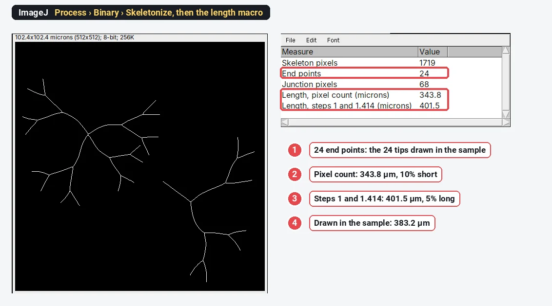
Neurite length and branching in ImageJ: Skeletonize and Analyze Skeleton
Neurite length and branching in ImageJ: threshold, Process › Binary › Skeletonize, then Analyze Skeleton (Fiji) or a macro. Why diagonal steps matter.
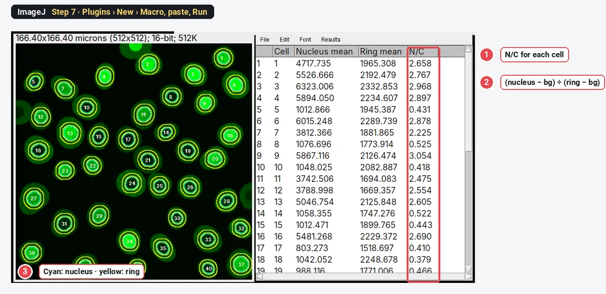
Nuclear/cytoplasmic ratio in ImageJ: quantify NF-κB, YAP or TFEB translocation
Measure the nuclear/cytoplasmic ratio in ImageJ step by step: nuclei from DAPI, a cytoplasm ring with Enlarge and Make Band, and an N/C table per cell.
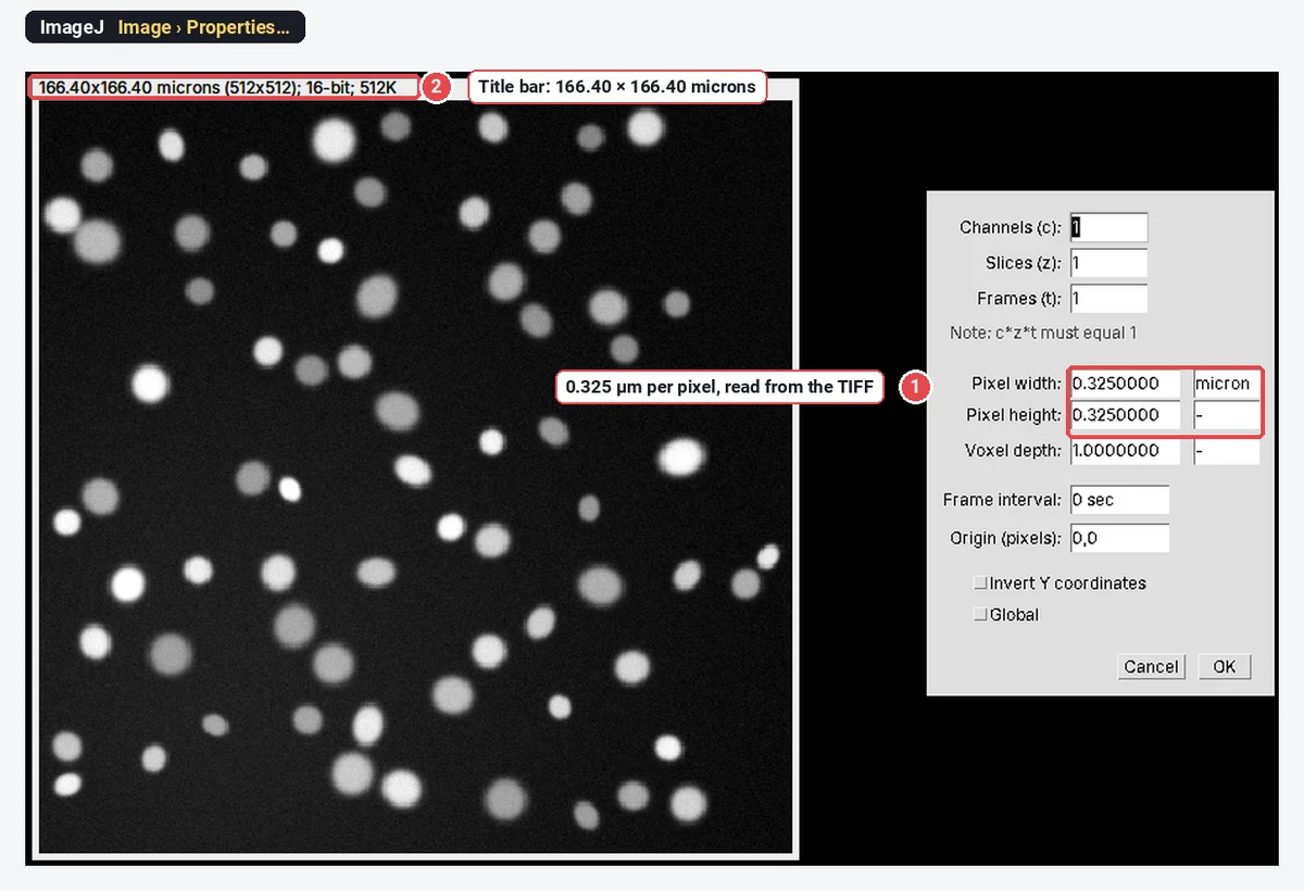
How to open .czi, .nd2, .lif and other microscope files in ImageJ (Bio-Formats)
Open Zeiss .czi, Nikon .nd2 and Leica .lif files in ImageJ with Bio-Formats (built into Fiji), keep the pixel size, and fix "Unsupported format".
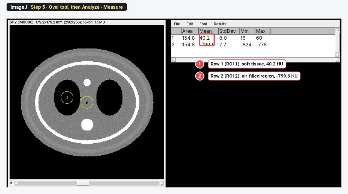
Open DICOM files in ImageJ (and a series as a stack)
Open DICOM files in ImageJ with File › Open, a whole series as a stack with Import › Image Sequence, read the tags, measure HU, and open compressed DICOM.
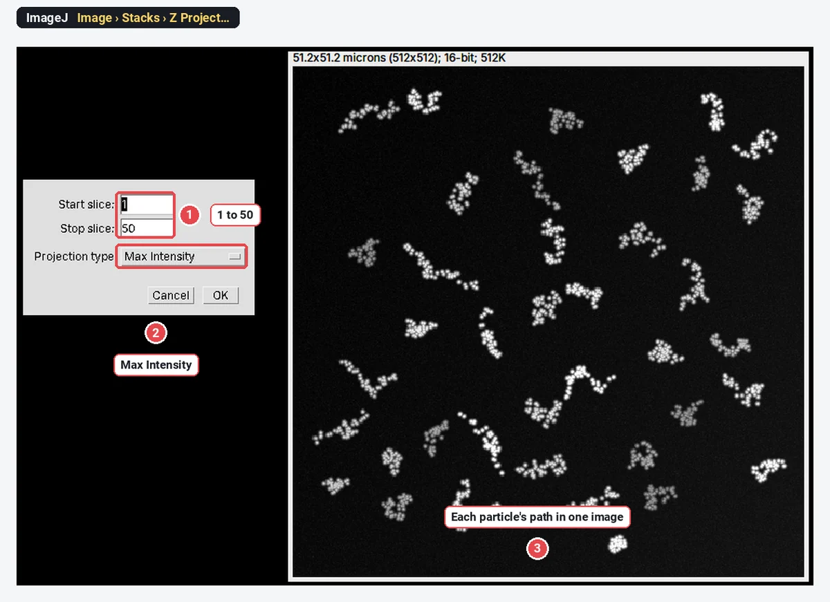
Particle tracking in ImageJ (TrackMate) and MSD: a practical guide
Track particles in ImageJ with TrackMate (Fiji) or Find Maxima, then get the diffusion coefficient from the MSD: MSD = 4Dt in 2D, with a worked example.
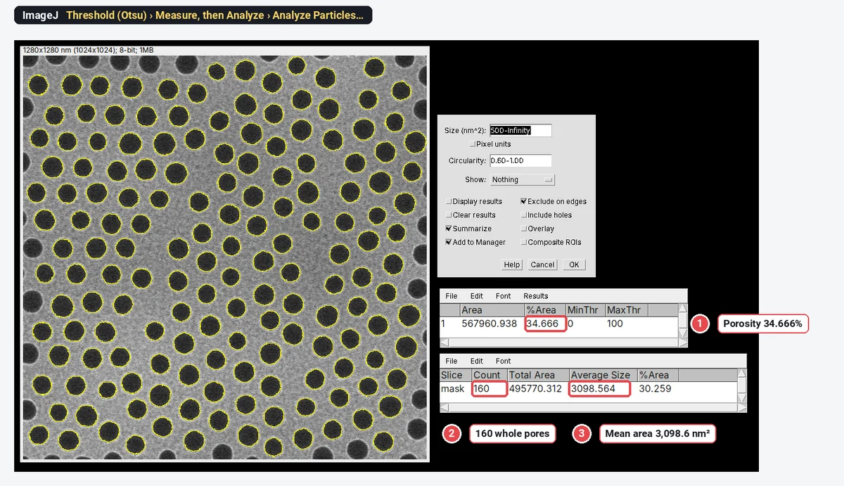
Porosity and pore size from SEM images in ImageJ (AAO, membranes, coatings)
Porosity and pore size from an SEM image in ImageJ: threshold the pores, read %Area as porosity, then Analyze Particles for pore areas and diameters.
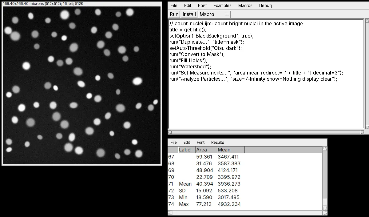
Use ImageJ from Python with PyImageJ (a gentle start)
Install PyImageJ, start ImageJ from Python with imagej.init, run your ImageJ macro, and get the image as NumPy and the Results table as pandas.
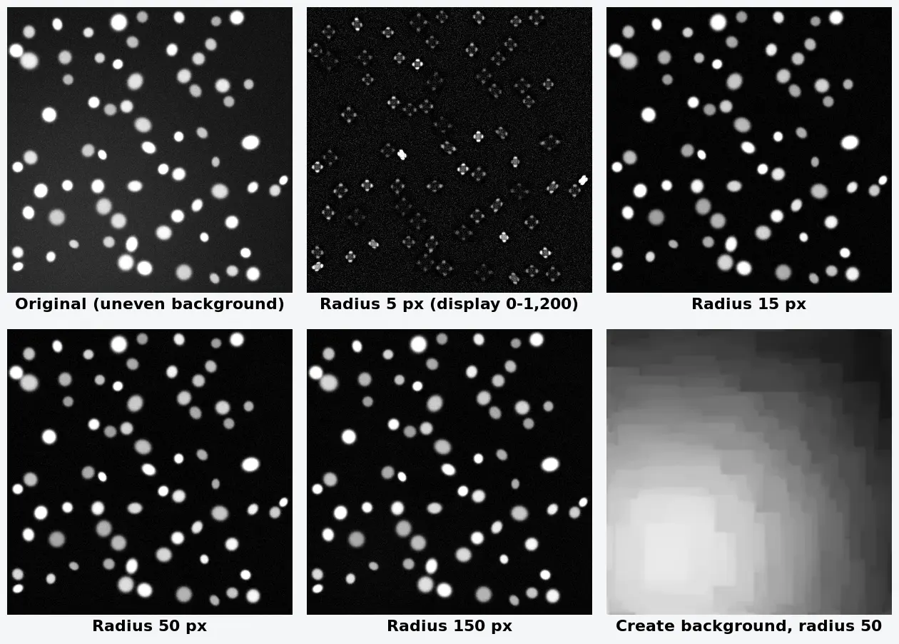
Rolling-ball background subtraction in ImageJ: how to choose the radius
Subtract background in ImageJ: Process › Subtract Background, a rolling ball radius at least the largest object's, Light background off for fluorescence.
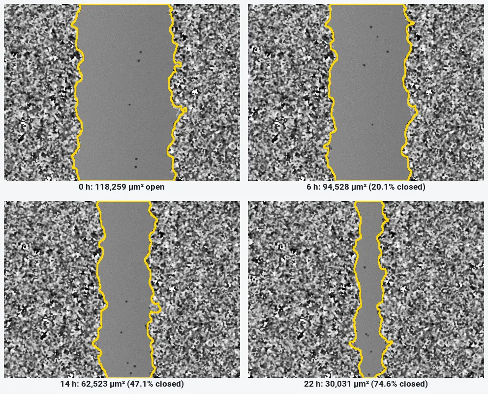
Wound healing (scratch) assay analysis in ImageJ: % closure step by step
Measure a scratch wound in ImageJ: variance filter, threshold and Analyze Particles per frame, then % closure and closure rate, with a worked example.
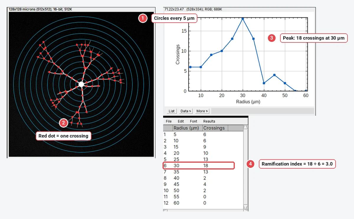
Sholl analysis in ImageJ/Fiji and online (step by step)
Sholl analysis step by step: circles around the cell body, crossings per radius, the Sholl plot, critical radius and ramification index, in Fiji (SNT) or with an ImageJ macro.
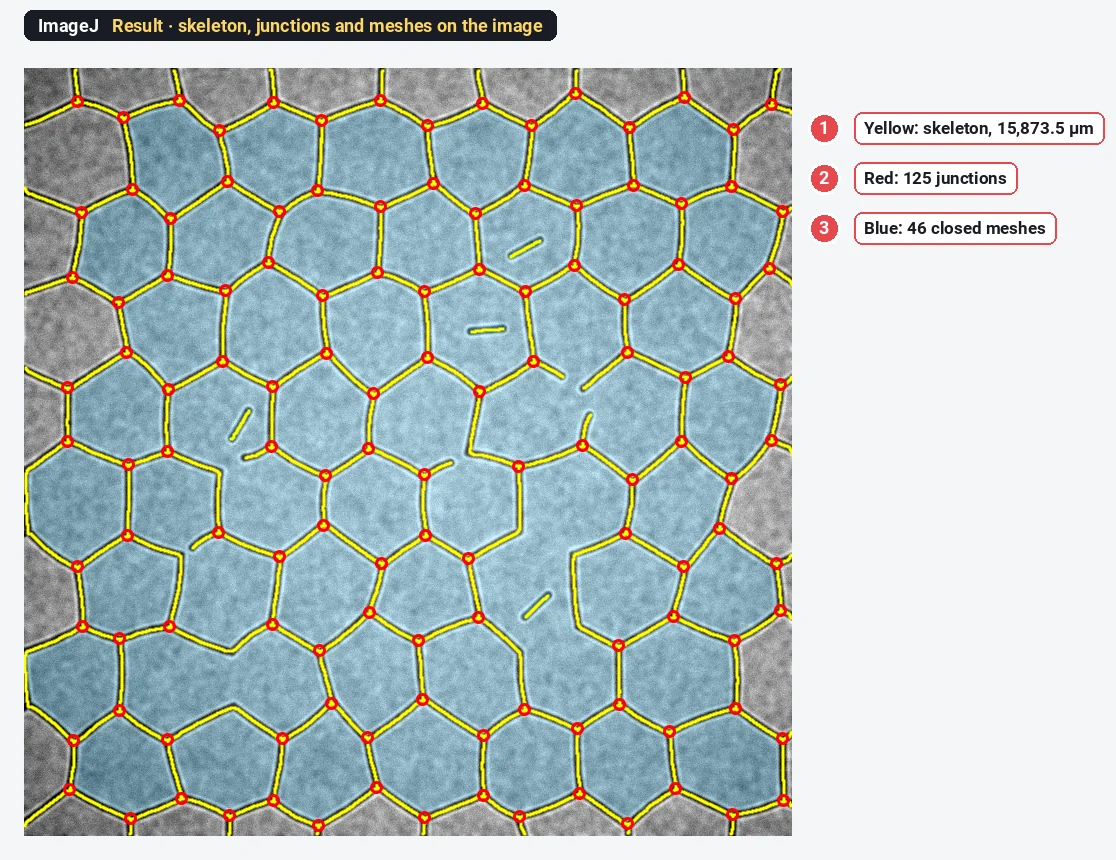
Tube formation assay quantification in ImageJ (and the Angiogenesis Analyzer)
Quantify a tube formation assay in ImageJ step by step: total tube length, junctions, segments and meshes, plus the Angiogenesis Analyzer and AngioTool.
Watershed in ImageJ: separate touching particles (and when not to)
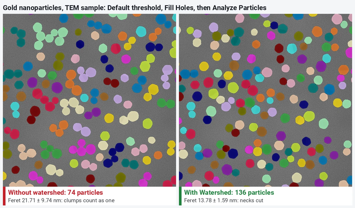
Split touching nuclei and nanoparticles with Process › Binary › Watershed in ImageJ, with before and after counts, and why it cuts nanorods to pieces.