How to make a kymograph in ImageJ and measure velocities
Make a kymograph in ImageJ: a line along the track, Image › Stacks › Reslice, then a line on each streak gives velocity = Δx ÷ Δt, with a worked example.
Contents
To make a kymograph in ImageJ, open the time-lapse, draw a line along the track (the Segmented Line tool for a curved axon or filament) and choose Image › Stacks › Reslice… (/): the new image has distance along the line across and one row per frame down, so every moving particle draws a sloped streak. To get a velocity, draw a straight line along a streak and measure how far it goes across (
Below: the steps in ImageJ and Fiji on a worked example with known speeds, the formula with its units, how to read the angle, and the Fiji plugins people use (KymoResliceWide, KymographBuilder, KymographClear). The time-lapse is synthetic: five particles moving along a curved filament at +1.0, −0.6, +0.4, 0 and −1.4 µm/s, 60 frames 0.5 s apart, 0.16 µm per pixel. Knowing the true speeds lets you see how close the measurement gets.
What is a kymograph?
A kymograph is a space-time picture of one line in a movie. Take the pixels along a line in frame 1 and lay them out as the top row; frame 2's pixels go in the second row, and so on. Distance along the line runs across, time runs down. Something that stays put draws a vertical streak, something moving towards the end of the line draws a streak leaning one way, and something moving back leans the other way. The slope of a streak is its speed.
Kymographs are the standard way to measure axonal and dendritic transport, motor proteins on microtubules, actin flow, growth-cone advance and anything else that moves along a known path. They work when movement is mostly along one line; for particles that wander in two dimensions, track them instead (see particle tracking and MSD).
How do I make a kymograph in ImageJ (or Fiji)?
Reslice is part of ImageJ 1.x, so these steps work in plain ImageJ and in Fiji.
- Open the time-lapse and check Image › Properties…: the pixel size (µm) and the Frame interval (s). If they are missing, set them now, or keep the numbers to hand.
- Find the track. If the filament or axon is faint, make a Max Intensity projection over time (Image › Stacks › Z Project…): every place a particle visited lights up. Draw your line on the projection, then move it to the movie with Edit › Selection › Restore Selection (Ctrl Shift E).
- Draw the line from the start of the track to its end, along it. Use the Segmented Line tool (right-click the line tool to choose it): click along the track, double-click to finish. Direction matters: the start of the line is the left edge of the kymograph.
- Image › Stacks › Reslice… (the / key). For a line selection the dialog offers Start at (Top puts frame 1 at the top), Flip vertically, Rotate 90 degrees and Avoid interpolation. Keep Start at: Top and Avoid interpolation ticked.
- OK. A new image opens, "Reslice of" plus the movie's name.
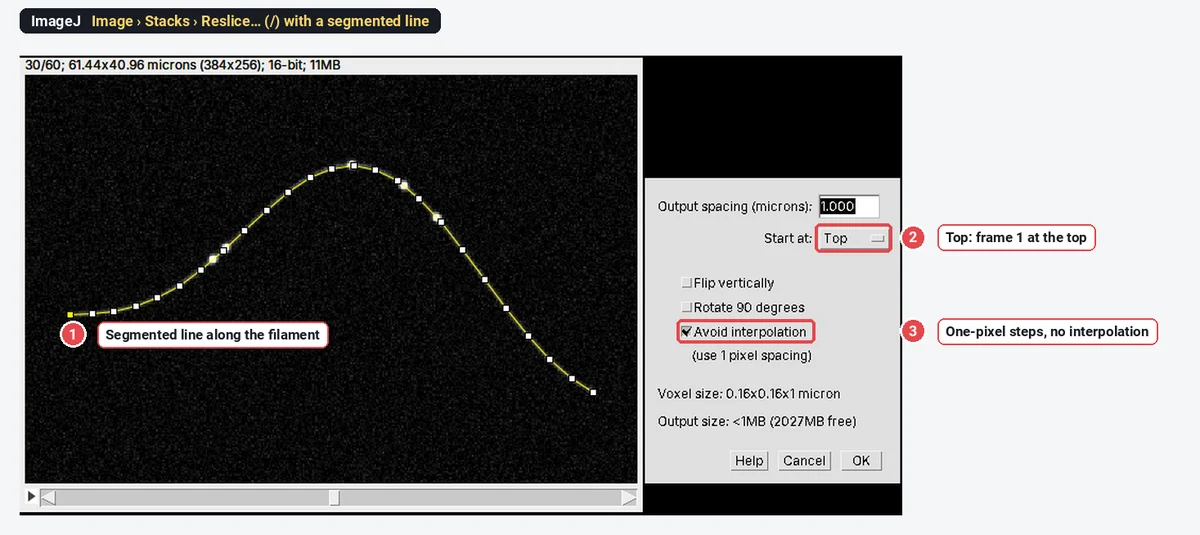
On the sample, the line is 66.89 µm long (the filament built into the sample is 66.9 µm), and Reslice returned a kymograph 417 pixels wide and 60 rows tall: one row per frame.
Make sense of the kymograph's units
The kymograph's x-axis is in the movie's pixels along the line: 0.16 µm each here. Its y-axis is in frames. ImageJ 1.54f labelled the rows with the movie's z-spacing (1 "micron" per row in our case), which is meaningless for time; the cleanest way to avoid confusion is Analyze › Set Scale… › Click to Remove Scale on the kymograph and to convert both axes yourself, as below.
How do I measure velocity from a kymograph?
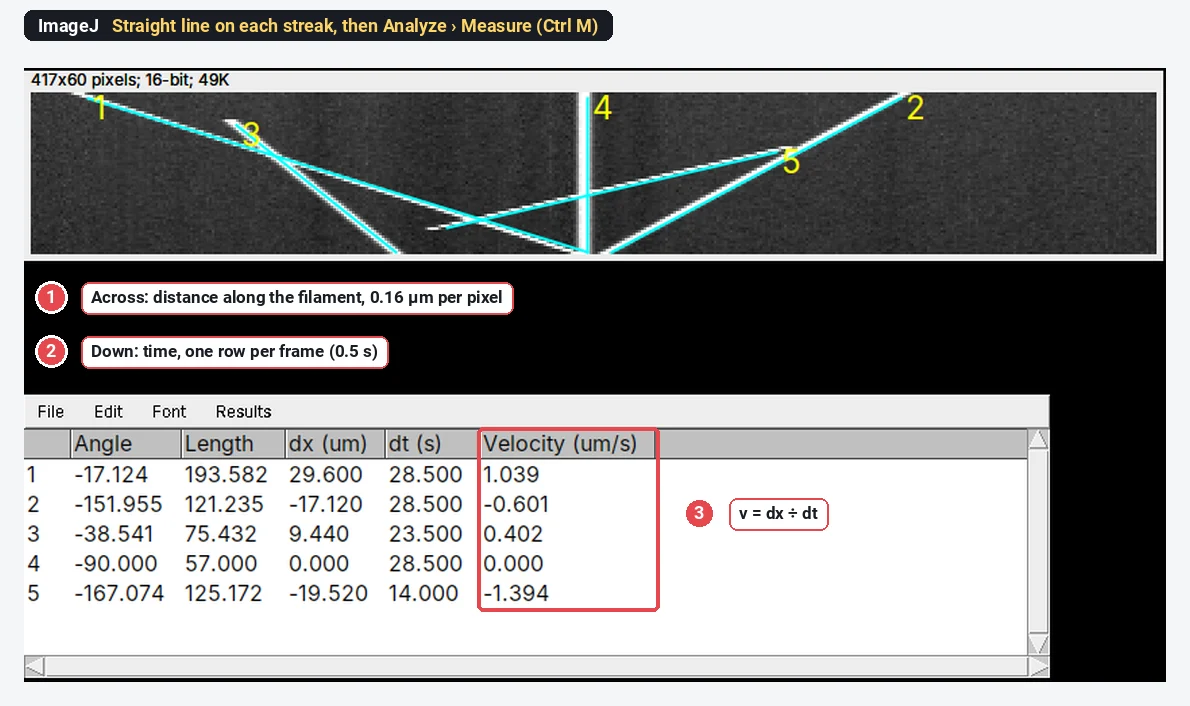
- Zoom in on the kymograph (it is only 60 rows tall here) and pick the Straight Line tool.
- Draw a line along one streak, from where it starts (top) to where it ends (bottom). Follow the middle of the streak; on a curved streak, measure the straight part you care about, or split it into runs.
- Press Ctrl M (Analyze › Measure). With a line selected, the Results table gives the Angle and Length.
- Add the next streak's line to the overlay (Image › Overlay › Add Selection, Ctrl B) so you can see what you have measured, and repeat.
- Convert.
With the angle
Here
The three extra columns came from a few lines of macro after measuring (px = 0.16 µm, dt = 0.5 s):
for (i = 0; i < nResults; i++) {
  a = getResult("Angle", i) * PI / 180; L = getResult("Length", i);
  dx = L * cos(a); dy = -L * sin(a);
  setResult("Velocity (um/s)", i, (dx * 0.16) / (dy * 0.5));
}
updateResults();
The worked example
| Streak | Across ( | Down ( | Velocity measured in ImageJ | Built into the sample |
|---|---|---|---|---|
| 1 | 185 px = 29.60 µm | 57 frames = 28.5 s | +1.039 µm/s | +1.0 µm/s |
| 2 | −107 px = −17.12 µm | 57 frames = 28.5 s | −0.601 µm/s | −0.6 µm/s |
| 3 | 59 px = 9.44 µm | 47 frames = 23.5 s | +0.402 µm/s | +0.4 µm/s |
| 4 | 0 px | 57 frames = 28.5 s | 0 | 0 (still) |
| 5 | −122 px = −19.52 µm | 28 frames = 14.0 s | −1.394 µm/s | −1.4 µm/s |
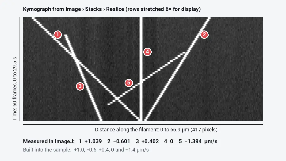
All five come within 4% of the truth. The small differences come from placing the line ends to the nearest pixel and from the 25-point line not following the smooth, curved filament exactly, so distances along it are not perfectly uniform. More points on the line, or a spline-fitted line (Edit › Selection › Fit Spline), help.
Reading the angle and the sign
ImageJ measures a line's Angle from the horizontal, counter-clockwise, with y pointing down the image. A line drawn from top to bottom therefore has a negative angle:
- Between 0 and −90° (leaning right): moving towards the end of your line, a positive velocity.
- −90° (vertical): not moving.
- Between −90 and −180° (leaning left): moving back towards the start, a negative velocity.
Which direction is "anterograde" depends only on which end you started the line from. Draw every line from the cell body outwards, or from the minus end to the plus end, and say so in the methods.
Units
| From | Multiply by | To |
|---|---|---|
| Pixels across | Pixel size (µm per pixel) | µm |
| Rows down | Frame interval (s per frame) | s |
| µm/s | 60 | µm/min |
Two limits follow from the units. The slowest speed you can see is about one pixel over the whole movie (
Wide lines and the Fiji kymograph plugins
Reslice in ImageJ 1.x samples a one-pixel path. In our test with ImageJ 1.54f it gave exactly the same kymograph from a 1-pixel and a 9-pixel-wide segmented line, so a wobbly axon that drifts off a thin line drops out of the kymograph. That is why Fiji users reach for plugins:
- KymoResliceWide (by Eugene Katrukha) works like Reslice but on wide straight, segmented and freehand lines, combining the pixels across the width, which follows a slightly wandering axon and averages away noise.
- KymographBuilder (by Hadrien Mary; Plugins › Kymograph › KymographBuilder in Fiji) builds a kymograph from a line on a time-lapse in one step.
- KymographClear is an ImageJ macro toolset that makes kymographs and colour-codes the directions of movement, and its companion KymographDirect extracts the streaks and their speeds automatically (Mangeol, Prevo and Peterman, 2016).
For a few streaks, hand-drawn lines in plain ImageJ are fine. For hundreds of vesicles with pauses and reversals, automated streak detection (KymographDirect, or tracking) saves days and is more reproducible.
Pitfalls
- No frame interval. Many exports lose it. A velocity off by the frame rate is off by a factor, silently. Check Image › Properties… against the acquisition software.
- A line that leaves the track. A one-pixel Reslice line on a moving axon misses particles. Draw on a Max projection over time, or use a wide-line tool.
- Lines drawn in both directions. The sign of every velocity flips with the line's direction.
- Fitting one line to a streak with pauses. A particle that runs, stops and runs again has no single velocity. Split the streak into runs and pauses, and report run speed, pause time and run length separately.
- Measuring on a kymograph you rescaled for display. Stretching the rows changes
- Only the clear streaks. Faint or short streaks are easy to skip and they are often the slow ones. Decide in advance what counts as a streak.
Reporting it
A methods sentence to copy:
Kymographs were generated in [Fiji (ImageJ 1.54f)] with Image › Stacks › Reslice along [segmented] lines drawn [from the soma towards the axon tip] on [maximum projections over time]. Velocities were calculated from straight lines traced along individual streaks as Δx ÷ Δt ([0.16] µm per pixel, [0.5] s per frame); [n] streaks from [n] cells.
Give the pixel size, frame interval, the line direction and how streaks were chosen, and show a kymograph with its distance and time scale bars. Cite ImageJ or Fiji, and the plugin if you used one.
An easier way: kymographs in LabCanvas
The Assays tab of LabCanvas Image Analysis has a Kymograph assay that does the same job in the browser, with nothing to install and no plugins, and this same transport sample built in.
- Open the time-lapse (or load the assay's sample) and choose the Channel to follow.
- Draw a line with the Line tool, click Trace a line to click points along a curved track, or let Find the track find the longest path along the bright structure of the time-averaged image.
- Set the Line width (the values are averaged across the width, unlike Reslice) and click Make kymograph.
- Draw lines along the streaks with the Line tool: each gets its velocity at once, in µm/s or µm/min (Speed in), and the summary counts how many move towards the end, towards the start or are still.
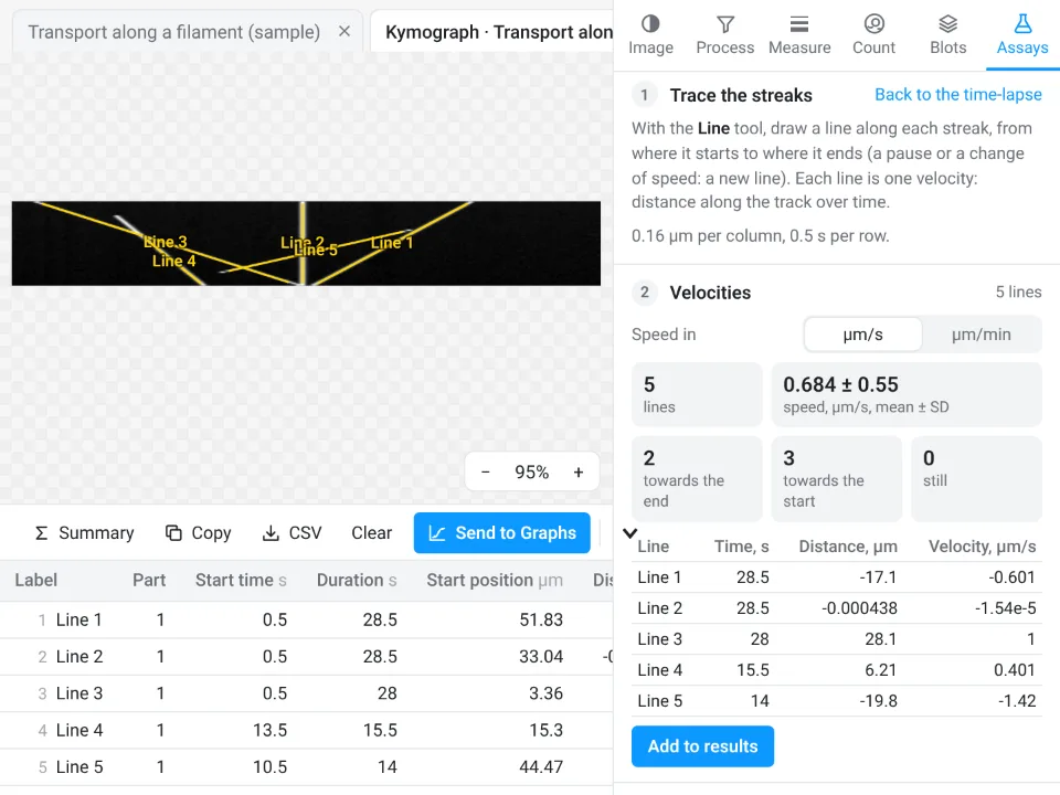
On the same five streaks, LabCanvas gave velocities from −1.42 to 1 µm/s; ImageJ's Reslice and Measure gave −1.394 to 1.039 µm/s; the true speeds are −1.4 to +1.0 µm/s.
Why it is a good choice for kymographs:
- Nothing to install, and a wide line out of the box, which plain ImageJ's Reslice does not do.
- Velocities without the arithmetic: no pixel size and frame interval to multiply by hand, and the direction of every streak is counted for you.
- Straight into Graphs: the table goes to Send to Graphs for a velocity plot, with a methods sentence to copy.
- Free with a LabCanvas account; downloading the kymograph as a TIFF or PNG is part of LabCanvas Pro. The measurements are checked in more than 4,000 automated tests.
For particles that leave the line, the Track assay links spots between frames and fits the mean squared displacement instead. Fiji is the better choice when you need automatic streak detection over many kymographs, or a macro that makes kymographs from hundreds of movies. Open Image Analysis, go to Assays › Kymograph and load the sample. ImageJ and Fiji are independent open-source projects; LabCanvas is not affiliated with them.
References
- Mangeol P, Prevo B, Peterman EJG (2016). KymographClear and KymographDirect: two tools for the automated quantitative analysis of molecular and cellular dynamics using kymographs. Molecular Biology of the Cell 27(12), 1948–1957. doi:10.1091/mbc.E15-06-0404
- Schneider CA, Rasband WS, Eliceiri KW (2012). NIH Image to ImageJ: 25 years of image analysis. Nature Methods 9, 671–675. doi:10.1038/nmeth.2089
- Schindelin J, Arganda-Carreras I, Frise E, et al. (2012). Fiji: an open-source platform for biological-image analysis. Nature Methods 9, 676–682. doi:10.1038/nmeth.2019
Frequently asked questions
How do I make a kymograph in ImageJ?
Open the time-lapse, draw a line along the path the particles take (Segmented line tool for a curved track), and choose Image › Stacks › Reslice… (the / key). With Start at: Top, the result has distance along the line across and one row per frame down: a kymograph.
How do I calculate velocity from a kymograph?
Draw a straight line along a streak and measure it. The streak covers
Why is a steep streak slow?
With time running down the kymograph, a particle that barely moves draws a nearly vertical streak, and a fast one draws a flat, shallow streak. A perfectly vertical streak is a particle standing still; a horizontal one would have moved the whole line in one frame.
Can I make a kymograph with a wide line in ImageJ?
Not with Reslice in ImageJ 1.54f: in our test it gave the same kymograph from a 1-pixel and a 9-pixel-wide line. Fiji users add KymoResliceWide, which builds the kymograph from a wide straight, segmented or freehand line, or use KymographBuilder.
What frame rate do I need for a kymograph?
Fast enough that a particle moves less than about its own size between frames, or its streak breaks into dots you cannot follow. At 0.16 µm pixels and 0.5 s frames, 1.4 µm/s is about 4 pixels per frame, still a continuous streak. Slow movement needs long recordings instead: the slowest you can measure is about one pixel over the whole movie.
Try it in LabCanvas
Every app is free to start in your browser. Create an account and begin.
Start Image Analysis free in your browserKeep reading
ImageJ vs LabCanvas Image Analysis: an honest comparison
ImageJ/Fiji or LabCanvas Image Analysis? Six everyday jobs done in both, six newer ones (macros, vendor files, 3D, StarDist, big images) and which to use.
How to use ImageJ: a beginner's tutorial for the 10 everyday jobs (2026)
How to use ImageJ and Fiji: get started, open an image, then 10 everyday jobs (scale, measure, threshold, count, background, blots) with exact menu paths.
How to set the scale and add a scale bar in ImageJ (with a calibration image to practise on)
Set the scale in ImageJ (Analyze › Set Scale) from a micrometer, scale bar or pixel size, add a scale bar, and practise on a free calibration image.