Neurite length and branching in ImageJ: Skeletonize and Analyze Skeleton
Neurite length and branching in ImageJ: threshold, Process › Binary › Skeletonize, then Analyze Skeleton (Fiji) or a macro. Why diagonal steps matter.
Contents
To measure neurite length and branching in ImageJ, threshold the neurites into a binary mask, run Process › Binary › Skeletonize to thin them to one-pixel lines, then measure the skeleton: Fiji's Analyze Skeleton (2D/3D) counts branches, junctions and end points and gives branch lengths, while in plain ImageJ a short macro adds up the length. Count diagonal steps as
length ≈ (straight steps × 1 + diagonal steps × 1.414) × pixel size
This guide works through the steps on a sample image with the numbers ImageJ gave, and explains what Fiji's Analyze Skeleton reports.
The sample: two branched cells
The worked example is a synthetic image made for these guides, saved as an ImageJ TIFF: 512 × 512 pixels at 0.2 µm per pixel, two branched cells in green fluorescence with processes that fork in two, thin and dim towards their tips, on an uneven background with noise. Because it was drawn from known paths, the answer is known: 24 end points, 17 branch points (12 in the first cell, 5 in the second) and 383.2 µm of processes measured from the cell centres.
A skeleton is the centre line of a shape, one pixel wide, that keeps its branching pattern: every process becomes a line, every fork a junction, every tip an end point.
Skeletonize in ImageJ, step by step
Process › Binary › Skeletonize is part of ImageJ 1.x, so it is the same in plain ImageJ and Fiji. It works only on binary images, so the threshold comes first.
- Check the scale: Image › Properties… should show µm per pixel (0.2 here). Set it with Analyze › Set Scale… if needed.
- Smooth a little if the outlines are ragged: Process › Filters › Gaussian Blur…, sigma 1 pixel. Bumps on the outline turn into spurs in the skeleton.
- Threshold: Image › Adjust › Threshold… (Ctrl Shift T). Pick a method, tick Dark background for bright neurites on a dark background, and check that the red overlay follows the processes out to their thin tips without the background. Otsu does on this image.
- Apply, or Process › Binary › Convert to Mask: the neurites become 255 and the rest 0.
- Clean the mask: Process › Binary › Fill Holes, and remove debris (Analyze Particles with a minimum size and Show: Masks gives a mask of the large objects only).
- Process › Binary › Skeletonize. Each object is thinned to a line one pixel wide.
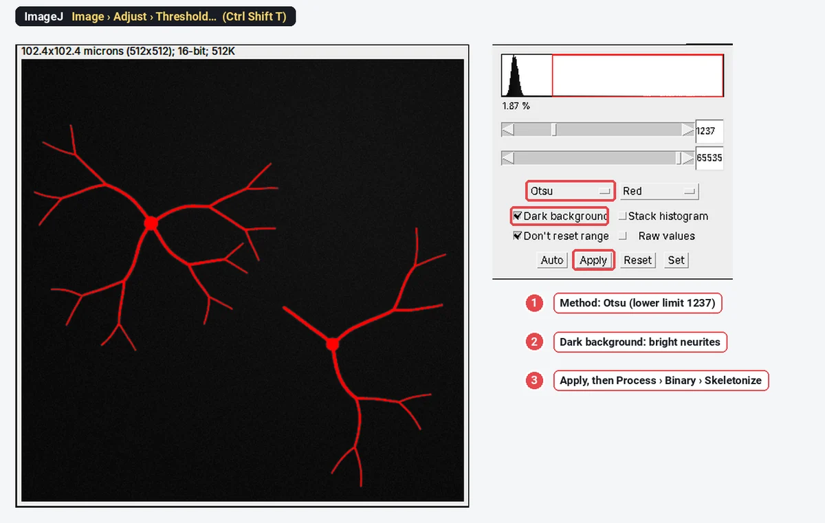
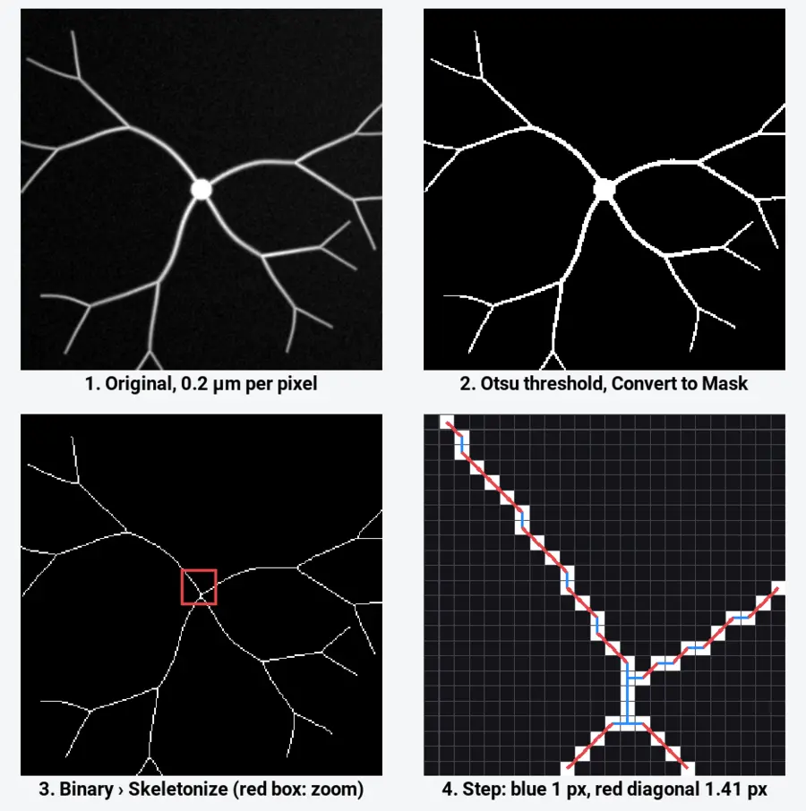
ImageJ's skeletonize is a thinning in the style of Zhang and Suen (1984): it peels pixels off the edges of each object, two sub-passes at a time, until only a connected line remains, keeping end points and connectivity. Lines in the result are 8-connected: neighbours can touch at a corner, which is where diagonal steps come from.
Measure the skeleton's length in plain ImageJ
ImageJ 1.x has no command that reports a skeleton's length, but two counts get you there.
The quick estimate: count the pixels. Select the skeleton image and use Analyze › Histogram (the count at 255) or Analyze › Measure with Integrated density in Set Measurements (
The better estimate: weight the steps. The macro below walks the skeleton, counts straight links (left-right, up-down) as 1 and diagonal links as
// Skeleton length, end points and junction pixels (ImageJ 1.x macro).
// Run it on the output of Process > Binary > Skeletonize.
getPixelSize(unit, pw, ph);
w = getWidth(); h = getHeight();
n = 0; orth = 0; diag = 0; ends = 0; junctions = 0;
for (y = 0; y < h; y++) {
  for (x = 0; x < w; x++) {
    if (getPixel(x, y) != 255) continue;
    n++;
    nb = 0;
    for (dy = -1; dy <= 1; dy++)
      for (dx = -1; dx <= 1; dx++)
        if ((dx != 0 || dy != 0) && getPixel(x + dx, y + dy) == 255) nb++;
    if (nb == 1) ends++;
    if (nb >= 3) junctions++;
    // links to the right and down: straight steps count 1, diagonal steps 1.414
    if (getPixel(x + 1, y) == 255) orth++;
    if (getPixel(x, y + 1) == 255) orth++;
    if (getPixel(x + 1, y + 1) == 255 && getPixel(x + 1, y) != 255 && getPixel(x, y + 1) != 255) diag++;
    if (getPixel(x - 1, y + 1) == 255 && getPixel(x - 1, y) != 255 && getPixel(x, y + 1) != 255) diag++;
  }
}
Table.create("Skeleton length");
Table.set("Measure", 0, "Skeleton pixels");       Table.set("Value", 0, n);
Table.set("Measure", 1, "End points");            Table.set("Value", 1, ends);
Table.set("Measure", 2, "Junction pixels");       Table.set("Value", 2, junctions);
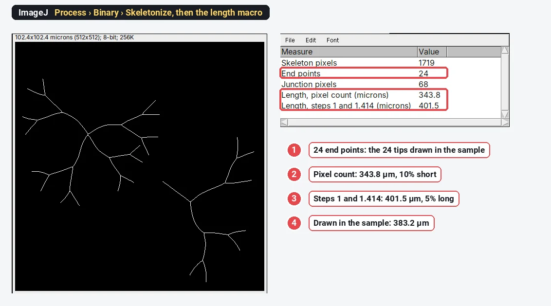
Table.set("Measure", 3, "Length, pixel count (" + unit + ")");    Table.set("Value", 3, d2s(n * pw, 1));
Table.set("Measure", 4, "Length, steps 1 and 1.414 (" + unit + ")"); Table.set("Value", 4, d2s((orth + diag * sqrt(2)) * pw, 1));
Table.update;
A diagonal link is only counted when no straight path joins the two pixels, so a corner made of two straight steps is not counted three times.
What the numbers say
| Estimate | Length on the sample | Against the drawn 383.2 µm |
|---|---|---|
| Pixel count × 0.2 µm | 343.8 µm | 10% short |
| Steps of 1 and 1.414 × 0.2 µm | 401.5 µm | 5% long |
The pixel count is short because diagonal stretches are undercounted. Weighted steps overshoot a little, because a smooth curve at a shallow angle becomes a staircase of straight and diagonal steps that is longer than the curve itself, and junctions add a few extra links where several pixels meet. Both errors are systematic: they are the same for treated and control images with the same magnification, so comparisons hold, but the absolute number depends on the method. Say which you used.
The end points come out right, 24, the number of tips in the drawing. The 68 junction pixels are not 17 branch points: at each fork several pixels have three or more neighbours, and they need grouping into one junction. That grouping, and the split into branches, is what Analyze Skeleton does.
Analyze Skeleton (2D/3D) in Fiji
Analyze Skeleton (2D/3D) is a Fiji plugin by Ignacio Arganda-Carreras and colleagues (cite Arganda-Carreras et al. 2010); it is not in plain ImageJ 1.x. Its documentation lists it under Plugins › Skeleton, next to Skeletonize (2D/3D), Fiji's own thinning for 2D images and 3D stacks, which follows Lee, Kashyap and Chu (1994). Typing "skeleton" in Fiji's search bar finds both.
- Skeletonize the mask (Process › Binary › Skeletonize for 2D, or Skeletonize (2D/3D), which also takes stacks).
- Run Analyze Skeleton (2D/3D). Options include pruning loops (cycles) in the skeleton, and showing detailed information: a table of every branch.
- Read the results. For each skeleton (each connected piece), the summary gives the number of branches, junctions, end-point voxels, junction voxels, slab voxels, triple and quadruple points, and the average and maximum branch length. The detailed table lists each branch's calibrated length, the coordinates of its two ends and the straight-line (Euclidean) distance between them, whose ratio to the length is the tortuosity.
- A tagged image colours end points, junctions and slabs differently, so you can check the classification by eye.
Pixels are classified by their neighbours: one neighbour is an end point, two is a slab (part of a branch), three or more is a junction. Touching junction pixels are grouped into one junction, which is why the junction count is far smaller than the junction-pixel count. Branch lengths are measured along the skeleton in calibrated units, each step at its real length (1 or 1.414 pixel widths in 2D), so they do not have the pixel-count error.
For total neurite length per cell, sum the branch lengths of that cell's skeleton. For neurite outgrowth assays, divide by the number of cell bodies (counted separately, for example on a nuclear stain).
Skeletons have limits that tracing does not. For single neurons in crowded cultures, Fiji's SNT measures paths you trace semi-automatically and is the most accurate route; for 3D stacks, use Skeletonize (2D/3D); and for thousands of images, record the steps as a macro and run it with Process › Batch › Macro….
Pitfalls
- A poor mask. The skeleton follows the mask: gaps split one neurite into two, merged neighbours join them. Check the threshold overlay before skeletonising; threshold methods compares them.
- Spurs. Ragged outlines make short side branches that inflate branch and end-point counts. Smooth first and prune spurs of a few pixels.
- Cell bodies. A thick soma skeletonises into a short line or a small star, adding branches and length. Mask the bodies out, or subtract them, when you report neurite length only.
- Pixel counting. It undercounts diagonals by up to 29%. Weight the steps, or use Analyze Skeleton's branch lengths.
- Crossing neurites. In dense cultures, two neurites crossing make a junction that is not a branch point. Skeleton methods cannot tell the difference; tracing can.
- Resolution. A neurite one or two pixels wide thresholds unevenly and breaks up. Image at a pixel size of a third or less of the neurite width.
- Images of different magnification. Lengths in pixels, and the staircase error, change with pixel size. Compare like with like, in µm.
Reporting it
A methods sentence to copy, with the parts in brackets filled in:
Neurites were segmented in [Fiji (ImageJ 1.54f)] by [Gaussian blur (σ = 1 px) and Otsu thresholding], skeletonised (Process › Binary › Skeletonize) and analysed with AnalyzeSkeleton (Arganda-Carreras et al., 2010), pruning branches shorter than [1] µm. Total neurite length per cell was the sum of branch lengths divided by the number of [DAPI-stained nuclei]; [n] fields from [N] independent cultures were analysed.
Report the length per cell (or per field), the number of branch points and end points, and show one example image with its skeleton overlaid.
Next: measure dendritic complexity with Sholl analysis.
An easier way: neurite length in LabCanvas
The Branching and skeleton assay of LabCanvas Image Analysis does the threshold, the skeleton and the measurement in one panel, in the browser, with nothing to install and no plugins.
- Open the image (a TIFF with its µm scale, or set the scale) and choose Assays › Branching and skeleton.
- Pick the Channel with the structures; they are found with a threshold (Li by default) after smoothing, with a smallest object size and holes to fill.
- Set Prune spurs shorter than to drop the short side branches that bumps on the outline make.
- Click Analyse: the skeleton, junctions and end points are drawn on the image.
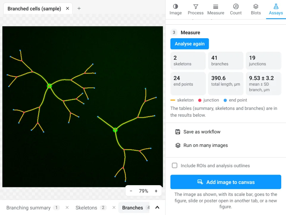
On the same sample: 2 skeletons, 41 branches, 19 junctions, 24 end points and a total length of 390.6 µm (2% above the drawn 383.2 µm), with branches of 9.53 ± 3.2 µm. ImageJ's macro gave the same 24 end points and 343.8 µm (pixel count) or 401.5 µm (weighted steps).
Why it is a good choice for neurite length:
- Nothing to install and no plugin to find: it runs in the browser on any computer or tablet.
- A guided assay instead of a threshold, Skeletonize and a macro: junctions are grouped and branch lengths measured along the skeleton, like Analyze Skeleton.
- The Branching summary, Skeletons and Branches tables (each branch with its length, straight-line distance and tortuosity) go straight to Graphs or a figure.
- A methods sentence to copy; free with a LabCanvas account (CSV download is part of Pro), and checked in more than 4,000 automated tests.
For 3D skeletons of stacks, traced reconstructions (SNT) and macro batch runs, ImageJ and Fiji remain the better tools. Open Image Analysis.
ImageJ and Fiji are independent open-source projects; LabCanvas is not affiliated with them.
References
- Arganda-Carreras I, Fernández-González R, Muñoz-Barrutia A, Ortiz-de-Solórzano C (2010). 3D reconstruction of histological sections: application to mammary gland tissue. Microscopy Research and Technique 73, 1019–1029. doi:10.1002/jemt.20829
- Zhang TY, Suen CY (1984). A fast parallel algorithm for thinning digital patterns. Communications of the ACM 27, 236–239. doi:10.1145/357994.358023
- Lee TC, Kashyap RL, Chu CN (1994). Building skeleton models via 3-D medial surface/axis thinning algorithms. CVGIP: Graphical Models and Image Processing 56, 462–478. doi:10.1006/cgip.1994.1042
- Schindelin J, Arganda-Carreras I, Frise E, et al. (2012). Fiji: an open-source platform for biological-image analysis. Nature Methods 9, 676–682. doi:10.1038/nmeth.2019
Frequently asked questions
How do I skeletonize an image in ImageJ?
Make the image binary first: Image › Adjust › Threshold…, choose a method, Apply (or Process › Binary › Convert to Mask). Then Process › Binary › Skeletonize thins every object to a line one pixel wide. Skeletonize only works on binary (8-bit, 0 and 255) images.
How do I measure neurite length in ImageJ?
Skeletonize the thresholded neurites and measure the skeleton. Counting skeleton pixels × pixel size underestimates diagonal stretches by up to 29%; counting straight steps as 1 and diagonal steps as
Where is Analyze Skeleton in Fiji?
Analyze Skeleton (2D/3D) comes with Fiji; its documentation lists it under Plugins › Skeleton, next to Skeletonize (2D/3D). Typing "Analyze Skeleton" in Fiji's search bar finds it whatever the menu layout. It is not part of plain ImageJ 1.x.
What does Analyze Skeleton measure?
It classifies every skeleton pixel as an end point (one neighbour), slab (two) or junction (three or more), groups touching junction pixels into junctions, and reports per skeleton the numbers of branches, junctions, end points, triple and quadruple points, and the average and maximum branch length. With the detailed-information option, it lists every branch with its length and end coordinates.
Why is my skeleton full of short spurs?
Bumps on the outline of the mask become short side branches when the shape is thinned. Smooth the image before thresholding (Process › Filters › Gaussian Blur, sigma 1–2 pixels), fill holes, and prune end branches shorter than a few pixels before you count.
Can I measure neurite length online?
Yes. The Branching and skeleton assay of LabCanvas Image Analysis thresholds, skeletonises and measures in the browser, with branches, junctions, end points and branch lengths; on our sample it gives 390.6 µm in total.
Try it in LabCanvas
Every app is free to start in your browser. Create an account and begin.
Start Image Analysis free in your browserKeep reading
ImageJ vs LabCanvas Image Analysis: an honest comparison
ImageJ/Fiji or LabCanvas Image Analysis? Six everyday jobs done in both, six newer ones (macros, vendor files, 3D, StarDist, big images) and which to use.
How to use ImageJ: a beginner's tutorial for the 10 everyday jobs (2026)
How to use ImageJ and Fiji: get started, open an image, then 10 everyday jobs (scale, measure, threshold, count, background, blots) with exact menu paths.
How to set the scale and add a scale bar in ImageJ (with a calibration image to practise on)
Set the scale in ImageJ (Analyze › Set Scale) from a micrometer, scale bar or pixel size, add a scale bar, and practise on a free calibration image.