Tube formation assay quantification in ImageJ (and the Angiogenesis Analyzer)
Quantify a tube formation assay in ImageJ step by step: total tube length, junctions, segments and meshes, plus the Angiogenesis Analyzer and AngioTool.
Contents
To quantify a tube formation assay in ImageJ, flatten the background (Process › Subtract Background…, Light background), smooth and threshold the tubes into a mask, skeletonize it (Process › Binary › Skeletonize) and measure the skeleton: its total length, its junctions (branch points) and the closed meshes between the tubes. Plain ImageJ 1.x has no command that counts junctions, so you either run the short macro below or install the Angiogenesis Analyzer toolset (Carpentier et al. 2020), which reports junctions, segments, branches, meshes and total length in one step.
The endothelial tube formation assay (HUVECs on Matrigel or another basement-membrane matrix, imaged after 4 to 18 hours) is the most common in-vitro angiogenesis test. The three numbers most papers report are total tube length, the number of junctions and the number of meshes.
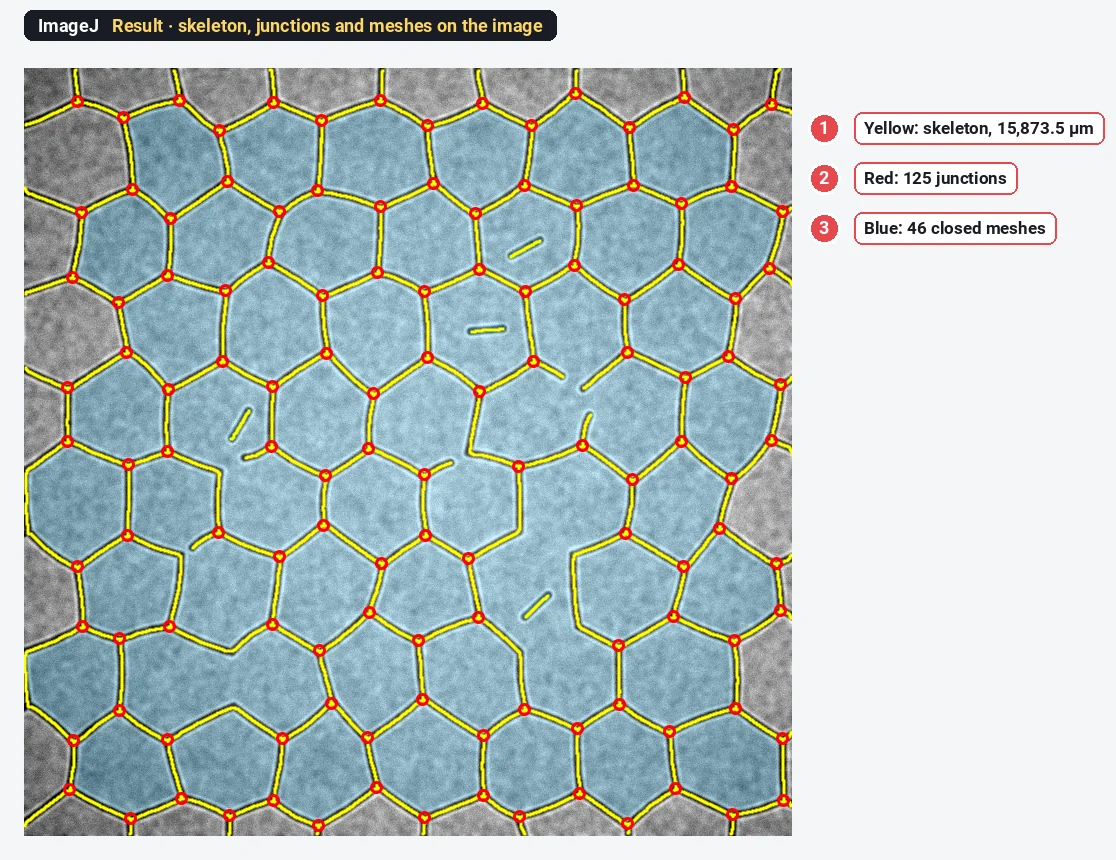
What you need: ImageJ 1.x or Fiji. A phase-contrast or fluorescence image of the network, ideally a TIFF with the pixel size. The example is a synthetic phase-contrast-like tube network made for practice: 768 × 768 pixels at 1.25 µm per pixel, dark tubes with a bright halo, darker corners, with a known 128 junctions, 172 segments and 46 closed meshes. Time: about 15 minutes.
What the numbers mean
| Measure | What it is |
|---|---|
| Total tube length | The summed length of the tube centre lines (the skeleton), in µm |
| Junction | A branch point where three or more tubes meet |
| Segment | A piece of tube between two junctions |
| Branch | A piece of tube with one free end |
| Mesh | A closed loop of tubes: an enclosed area of matrix |
| Isolated element | A tube not connected to the network |
A more mature network has more junctions and meshes and a longer total length; inhibitors of angiogenesis break the loops and leave short, isolated pieces.
How do I quantify tube formation in ImageJ? Step by step
Step 1: Flatten the background
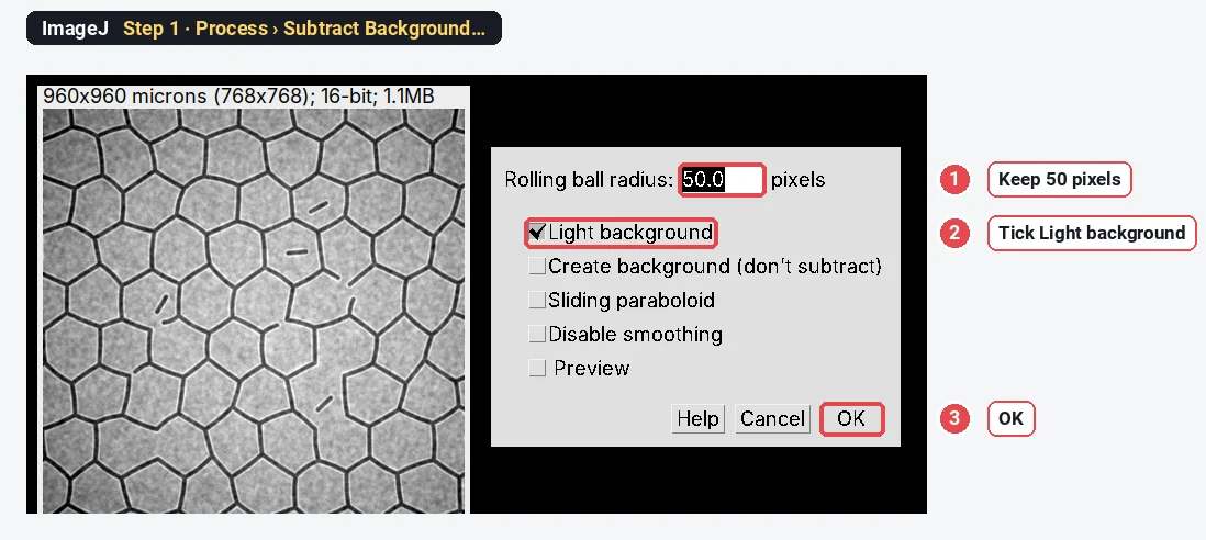
Open the image (File › Open…). Phase-contrast pictures are brighter in the centre than in the corners, and one threshold cannot handle that. Choose Process › Subtract Background…, keep Rolling ball radius 50 pixels (larger than the tube width), tick Light background (the tubes are darker than the matrix) and click OK.
Step 2: Smooth the noise
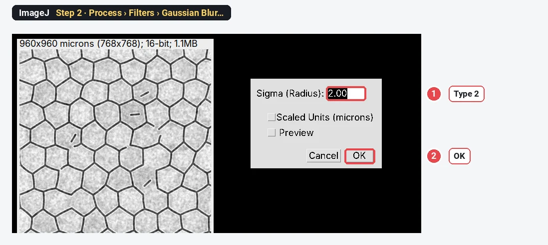
Choose Process › Filters › Gaussian Blur…, type 2 for Sigma and click OK. This evens out the matrix texture so the threshold makes clean tube edges.
Step 3: Threshold the tubes
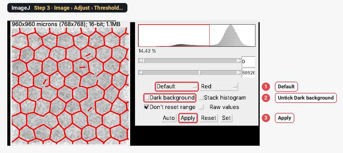
Open Image › Adjust › Threshold…. Choose Default, and make sure Dark background is not ticked, because here the objects (the tubes) are dark. The tubes turn red. Click Apply: the image becomes a black-and-white mask with white tubes.
Step 4: Remove the specks
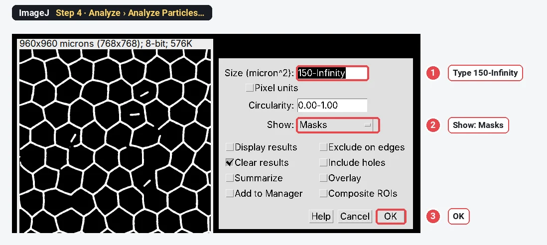
Choose Analyze › Analyze Particles…, type a size of 150-Infinity (µm²) and set Show to Masks. Click OK. ImageJ makes a new mask with only the tubes and pieces bigger than 150 µm², so dirt and texture do not become tiny tubes. If the new mask shows black tubes on white, choose Image › Lookup Tables › Invert LUT so the tubes look white.
Step 5: Skeletonize
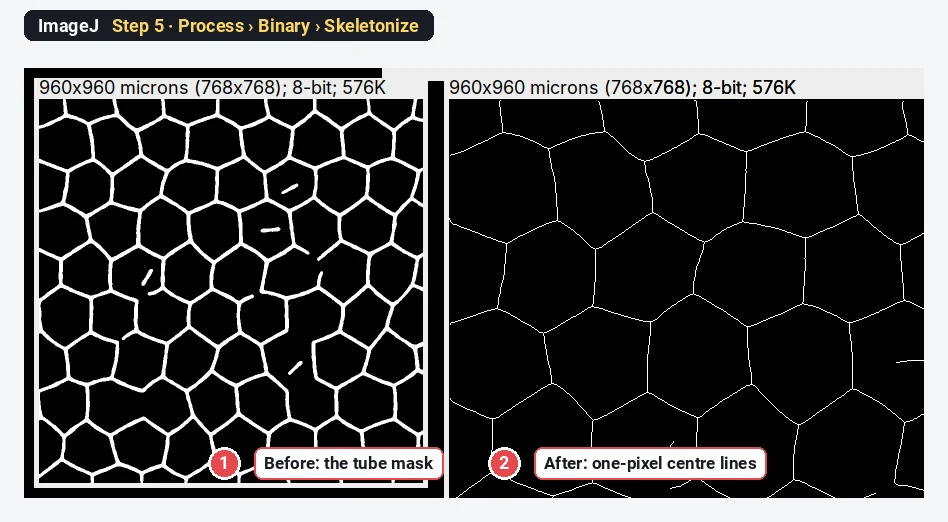
Make a copy of the clean mask with Image › Duplicate… (you need the mask again in Step 6). On the copy, choose Process › Binary › Skeletonize. Every tube shrinks to a line one pixel wide along its centre.
Step 6: Count the meshes
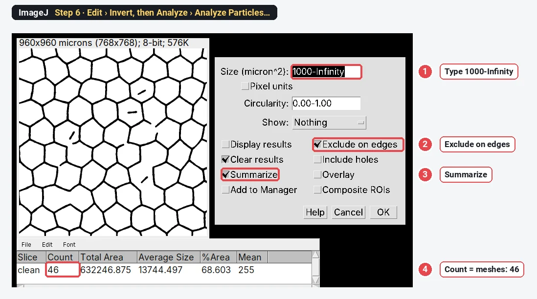
Click the clean mask (not the skeleton). Choose Edit › Invert, so the enclosed areas become white objects. Then Analyze › Analyze Particles… with a size of 1000-Infinity (µm²), Exclude on edges (an area cut by the frame is not a closed mesh) and Summarize ticked. The Count in the Summary window is the number of meshes: 46 here, the same as in the image's design.
Step 7: Measure length, junctions and segments with a macro
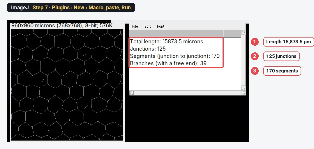
Click the skeleton window, choose Plugins › New › Macro, paste the code below and click Run. It walks along the skeleton and prints the total length, the junctions, the segments and the branches in the Log window. Diagonal steps count as
// Network measurements on a skeleton in plain ImageJ 1.x.
// Select the skeleton image (white lines on black, from Process › Binary › Skeletonize), then run.
// Diagonal steps count as √2 pixels; a junction is a branch point (3 or more neighbours);
// segments are the pieces of skeleton between two junctions, branches the pieces with a free end.
getPixelSize(unit, pw, ph);
skel = getImageID();
setBatchMode(true);
w = getWidth(); h = getHeight();
newImage("junctions", "8-bit black", w, h, 1); jun = getImageID();
newImage("ends", "8-bit black", w, h, 1); end = getImageID();
selectImage(skel);
len = 0;
for (y = 0; y < h; y++) for (x = 0; x < w; x++) {
  if (getPixel(x, y) == 0) continue;
  n = 0;
  for (dy = -1; dy <= 1; dy++) for (dx = -1; dx <= 1; dx++) {
    if ((dx != 0 || dy != 0) && getPixel(x + dx, y + dy) > 0) {
      n++;
      if (dx == 0 || dy == 0) len += 0.5; else len += 0.5 * sqrt(2);
    }
  }
  if (n == 1) { selectImage(end); setPixel(x, y, 255); selectImage(skel); }
  if (n >= 3) { selectImage(jun); setPixel(x, y, 255); selectImage(skel); }
}
// Junctions: touching branch-point pixels count as one junction.
selectImage(jun);
run("Analyze Particles...", "size=0-Infinity pixel show=Nothing clear");
junctions = nResults;
// Cut the skeleton at the junctions and sort the pieces.
run("Duplicate...", "title=cut"); run("Dilate");
imageCalculator("Subtract create", skel, "cut"); rename("pieces");
close("cut");
roiManager("reset");
run("Analyze Particles...", "size=0-Infinity pixel show=Nothing clear add");
pieces = roiManager("count"); branches = 0;
selectImage(end);
for (i = 0; i < pieces; i++) {
  roiManager("select", i);
  getStatistics(a, mean, min, max);
  if (max > 0) branches++;
}
run("Select None");
close("junctions"); close("ends"); close("pieces");
setBatchMode(false);
print("Total length: " + d2s(len * pw, 1) + " " + unit);
print("Junctions: " + junctions);
print("Segments (junction to junction): " + (pieces - branches));
print("Branches (with a free end): " + branches);
The macro expects a white skeleton on black: check that Process › Binary › Options › Black background is ticked before you make the masks.
The result on the sample
| Measure | ImageJ (this guide) | Built into the image |
|---|---|---|
| Total tube length | 15,873.5 µm | not given (the design runs past the frame) |
| Junctions | 125 | 128 |
| Segments | 170 | 172 |
| Branches with a free end | 39 | 40 |
| Meshes | 46 | 46 |
Meshes are exact; junctions and segments are within 2%. Skeleton methods tend to lose a few junctions: where two branch points lie very close, their pixels touch and are counted as one cluster, and short spurs can add false ones elsewhere. Every skeleton-based tool, the Angiogenesis Analyzer included, has some such error, so compare conditions analysed the same way rather than numbers from different tools.
Why flatten the background first?
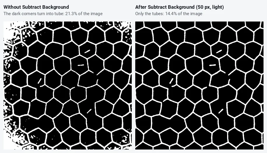
Phase-contrast and brightfield images are almost always darker at the corners (vignetting). A single threshold then either misses tubes in the bright centre or turns the dark corners into a solid web. The rolling ball removes the slow change in brightness and leaves the thin dark tubes. Its radius must be larger than the tube width; 50 pixels (62.5 µm) works here, where tubes are about 7 pixels wide.
The Angiogenesis Analyzer: the same job in one click
The Angiogenesis Analyzer is a macro toolset for ImageJ written by Gilles Carpentier and described in Carpentier et al. (2020). It was built for exactly this assay (and for the fibrin bead assay), and it reports, per image: nodes and junctions, extremities, branches, segments, isolated elements, meshes, total length, total branching length and total mesh area. Many published tube formation papers use it, which makes your numbers comparable with theirs.
To use it, download the toolset file from the author's page and put it in the macros/toolsets folder of ImageJ or Fiji. Restart, click the >> (More Tools) button at the right end of the toolbar and choose the Angiogenesis Analyzer: its buttons replace part of the toolbar, with separate analyses for phase-contrast and fluorescence images and a batch mode for a folder. It works in plain ImageJ 1.x as well as Fiji. We did not run it for this guide, so there is no screenshot; the steps above show what it does inside (background, segmentation, skeleton, junctions, meshes).
AngioTool (Zudaire et al. 2011) is a different program: a stand-alone Java tool from the US National Cancer Institute, made for vessel networks in tissue such as the retina. It reports vessel area, total and average vessel length, junctions, end points and lacunarity. For in-vitro tube formation, the Angiogenesis Analyzer is the more usual choice.
In Fiji, Analyze › Skeleton › Analyze Skeleton (2D/3D) (the AnalyzeSkeleton plugin) gives branches, junctions and branch lengths of any skeleton, which replaces the macro of Step 7.
Pitfalls
- Dark background ticked by mistake. The threshold then selects the matrix, not the tubes. The red must sit on the tubes.
- Short spurs. Rough tube edges grow tiny side branches when skeletonized; each adds a false junction. Smooth before thresholding, or prune branches shorter than a few pixels (the Angiogenesis Analyzer and AnalyzeSkeleton both have options for it).
- Clumps of cells. Cell aggregates make thick blobs whose skeleton is a tangle of junctions. Note them, or remove them from the mask by size or circularity before skeletonizing.
- Meshes cut by the frame. They are not closed, so exclude them, as in Step 6.
- The edge of the well. The meniscus makes a bright or dark ring; image the centre of the well, or crop the edge away.
- Different magnifications. Lengths scale with the pixel size, counts with the field size. Image every condition at the same magnification and report per field or per mm².
Reporting it
Tube formation was quantified in [Fiji (ImageJ 1.54)] on [4×] phase-contrast images ([n] fields per well). Background was removed with a rolling ball (radius [50] pixels, light background) and the image smoothed (Gaussian σ = [2] pixels); tubes were segmented with the [Default] threshold, objects < [150] µm² removed and the mask skeletonized. Total tube length and junctions were measured on the skeleton; meshes were counted as enclosed areas ≥ [1000] µm² not touching the image border. [Alternatively: analysed with the Angiogenesis Analyzer for ImageJ (Carpentier et al. 2020).]
Plot total length, junctions and meshes per condition, one point per well or experiment, normalised to the control if plates differ.
Switch to LabCanvas: tube formation in a few clicks
The same analysis runs in LabCanvas Image Analysis in the browser: no toolset to install, no macro.
- Open your image and go to the Assays tab › Tube formation (or click Try it on a sample).
- Under Find the tubes, check the outline on the image (background flattening is built in).
- Under Network, set Prune sprouts shorter than and Smallest mesh.
- Under Measure, read total length, segments, branches, junctions and meshes, and send them to Graphs.
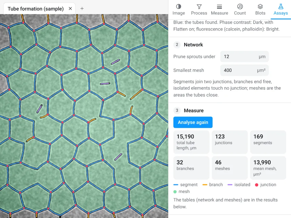
On the same synthetic network, LabCanvas gives 15,190 µm total length, 123 junctions, 169 segments and 46 meshes; ImageJ with the steps above gives 15,873.5 µm, 125 junctions, 170 segments and 46 meshes. The image was built with 128 junctions, 172 segments and 46 meshes. The lengths differ by about 4%: the two tools trace the centre lines and trim short spurs a little differently, so keep one tool for a whole study.
Why switch for tube formation:
- No toolset, no macro: junctions, segments and meshes come from one panel, with the network drawn on the image.
- Pruning built in: short sprouts and small meshes are left out by settings, the same for every image.
- Straight to Graphs: every parameter per image to a graph with statistics, and a methods sentence to copy.
The Angiogenesis Analyzer stays the reference if you need its exact parameter set to compare with published work, and Fiji is better for large batches through macros.
Open Image Analysis: free with a LabCanvas account (downloading CSV and image files is part of LabCanvas Pro). ImageJ and Fiji are independent open-source projects; LabCanvas is not affiliated with them.
References
- Carpentier G, Berndt S, Ferratge S, Rasband W, Cuendet M, Uzan G, Albanese P (2020). Angiogenesis Analyzer for ImageJ: a comparative morphometric analysis of "Endothelial Tube Formation Assay" and "Fibrin Bead Assay". Scientific Reports 10, 11568. doi:10.1038/s41598-020-67289-8
- Zudaire E, Gambardella L, Kurcz C, Vermeren S (2011). A computational tool for quantitative analysis of vascular networks. PLoS ONE 6, e27385. doi:10.1371/journal.pone.0027385
- Schindelin J, Arganda-Carreras I, Frise E, et al. (2012). Fiji: an open-source platform for biological-image analysis. Nature Methods 9, 676–682. doi:10.1038/nmeth.2019
- Schneider CA, Rasband WS, Eliceiri KW (2012). NIH Image to ImageJ: 25 years of image analysis. Nature Methods 9, 671–675. doi:10.1038/nmeth.2089
Frequently asked questions
How do I quantify a tube formation assay in ImageJ?
Flatten the background (Process › Subtract Background, Light background), smooth lightly, threshold the tubes and make a mask, remove specks with Analyze Particles (Show: Masks), then Process › Binary › Skeletonize. Total tube length comes from the skeleton, junctions are skeleton pixels with three or more neighbours, and meshes are the closed holes of the network counted with Analyze Particles on the inverted mask. The Angiogenesis Analyzer toolset does all of this in one click.
What is the Angiogenesis Analyzer for ImageJ?
A free macro toolset for ImageJ by Gilles Carpentier, described by Carpentier et al. (2020) in Scientific Reports. It analyses phase-contrast or fluorescence images of tube formation assays and reports nodes, junctions, extremities, branches, segments, meshes, total length and mesh area for each image. It is installed as a toolset and runs in ImageJ 1.x and Fiji.
Which parameters should I report for a tube formation assay?
Total tube length, the number of junctions (branch points) and the number of meshes (closed loops) are the most used and the most robust. Number of segments and total mesh area add detail. Normalise to the field area if fields differ, and report means of independent experiments.
What is the difference between a segment and a branch?
In the Angiogenesis Analyzer vocabulary, a segment is a piece of tube between two junctions, and a branch is a piece that ends freely on one side. Isolated elements are tubes not connected to anything. Our macro reports segments and branches the same way.
Is AngioTool the same as the Angiogenesis Analyzer?
No. AngioTool (Zudaire et al. 2011) is a separate stand-alone Java program from the US National Cancer Institute, written for vessel networks in tissue (retina, hindbrain, allantois). It reports vessel area, total and average vessel length, junctions, end points and lacunarity. The Angiogenesis Analyzer runs inside ImageJ and is built for in-vitro tube formation and fibrin bead assays.
Can ImageJ count junctions without a plugin?
Not with a menu command: plain ImageJ 1.x can skeletonize but has no command that counts branch points. The short macro in this guide does it by counting skeleton pixels with three or more neighbours. In Fiji, Analyze › Skeleton › Analyze Skeleton (2D/3D) reports branches, junctions and branch lengths.
Try it in LabCanvas
Every app is free to start in your browser. Create an account and begin.
Start Image Analysis free in your browserKeep reading
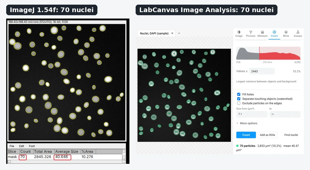
ImageJ vs LabCanvas Image Analysis: an honest comparison
ImageJ/Fiji or LabCanvas Image Analysis? Six everyday jobs done in both, six newer ones (macros, vendor files, 3D, StarDist, big images) and which to use.
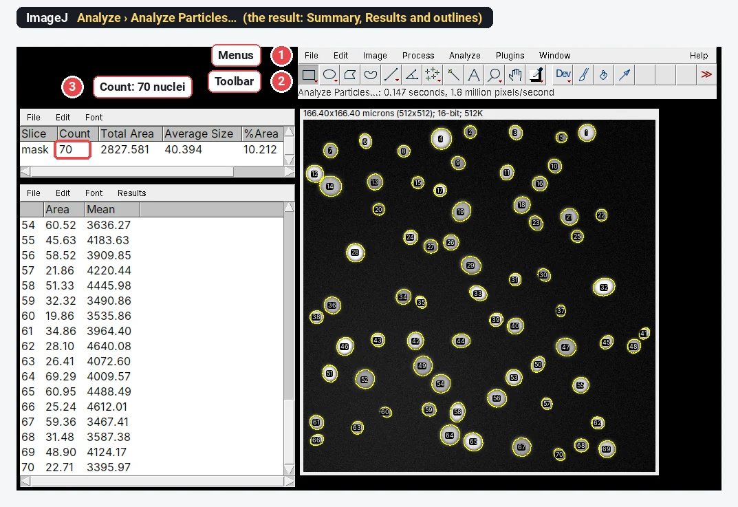
How to use ImageJ: a beginner's tutorial for the 10 everyday jobs (2026)
How to use ImageJ and Fiji: get started, open an image, then 10 everyday jobs (scale, measure, threshold, count, background, blots) with exact menu paths.
How to set the scale and add a scale bar in ImageJ (with a calibration image to practise on)
Set the scale in ImageJ (Analyze › Set Scale) from a micrometer, scale bar or pixel size, add a scale bar, and practise on a free calibration image.