Sholl analysis in ImageJ/Fiji and online (step by step)
Sholl analysis step by step: circles around the cell body, crossings per radius, the Sholl plot, critical radius and ramification index, in Fiji (SNT) or with an ImageJ macro.
Contents
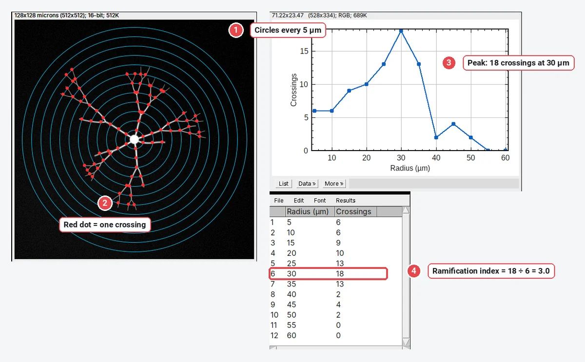
Sholl analysis counts how many times a neuron's branches cross a set of concentric circles centred on the cell body, and plots that count against the radius. In Fiji, threshold the neuron, mark the centre and run the Sholl Analysis command that comes with SNT; in plain ImageJ, a short macro on a binary mask does the same. The summary numbers are the maximum number of crossings, the radius where it occurs (the critical radius) and the ramification index:
For example,
This guide covers what the method measures, the Fiji route, a plain-ImageJ macro with the numbers it gave on a sample neuron, and how to read the Sholl plot.
What Sholl analysis measures
Donald Sholl described the method in 1953 to compare the dendrites of cat cortical neurons: draw circles at equal steps around the cell body and count the dendrites that cross each one. The count rises as branches split, peaks where the arbor is busiest, and falls to zero past the farthest tip. The resulting curve, the Sholl profile, is a compact description of dendritic complexity: how much branching there is, and how far from the soma it happens.
The numbers you report:
| Metric | Definition |
|---|---|
| Crossings N(r) | Number of branches crossing the circle of radius r |
| Maximum (critical value) | The largest N(r) |
| Critical radius | The radius at which N(r) is largest |
| Primary branches | Branches leaving the cell body (often read from the first circle) |
| Ramification index | Maximum ÷ primary branches (Schoenen's index) |
| Sum and mean | Total crossings over all circles, and their mean per circle; the sum depends on the step |
| Enclosing radius | The largest radius with at least one crossing |
| Sholl regression coefficient k | The slope of the semi-log fit, |
Sholl analysis needs the arbor of one neuron, segmented from its neighbours, with a sensible centre. It works on a thresholded image of a filled neuron (a fill, a sparse label, a Golgi stain) or on a tracing.
The sample neuron
The worked example uses a synthetic neuron made for these guides, saved as an ImageJ TIFF: 512 × 512 pixels at 0.25 µm per pixel, the cell body at the centre, 6 primary dendrites, 24 branch points and 30 tips, with dendrites that run outwards and thin and dim towards their tips, on an uneven background with noise. Because it was drawn from known paths, its true profile is known: 17 crossings at 30 µm is the maximum.
Sholl analysis in Fiji (SNT)
Fiji's Sholl Analysis began as a stand-alone plugin by Tiago Ferreira and colleagues (Ferreira et al. 2014) and is now part of SNT, Fiji's neuroanatomy toolbox (Arshadi et al. 2021). It is the most complete Sholl tool: it works on images in 2D and 3D and on traced reconstructions, and it fits the profile with polynomials and the semi-log and log-log methods.
- Install or update SNT: it comes with Fiji through the Neuroanatomy update site (Help › Update…, Manage update sites, tick Neuroanatomy), if it is not already there.
- Segment the neuron: Image › Adjust › Threshold…, pick a method that keeps the thin distal branches without the background (see threshold methods), and check the red overlay. Remove neighbouring cells with the eraser or a selection and Edit › Clear Outside.
- Mark the centre: a point on the cell body with the Point tool, or a straight line from the cell body outwards (its first point is the centre, its length can set the ending radius).
- Run Sholl Analysis: in recent Fiji it is listed with the other SNT commands (the Neuroanatomy shortcut window under Plugins › Neuroanatomy, and the Analysis menu). Menu names have moved between versions, so the quick way is to type Sholl in Fiji's search bar.
- Set the radii: Starting radius, Ending radius and Radius step size, in µm when the image is calibrated. A step of 1–10 µm is typical; the sum of crossings depends on it, the maximum and critical radius much less.
- Choose the outputs: the profile table, the plots (linear, semi-log, log-log), and the number of primary branches, which you can type in or have inferred from the first circle.
The results include the maximum, the critical radius, the ramification index, the enclosing radius and the regression coefficients. For 3D stacks, Fiji counts crossings on spheres, which plain ImageJ cannot do without much more code.
Sholl analysis in plain ImageJ: circles and a macro
Plain ImageJ 1.x has no Sholl command, but the measurement is simple enough for a macro: on a binary mask, walk round each circle and count every step from background into the neuron.
- Open the image and check the scale with Image › Properties… (0.25 µm here).
- Image › Adjust › Threshold…, method Otsu, Dark background ticked (bright neuron on dark background), then Process › Binary › Convert to Mask.
- With the Point tool, click the centre of the cell body.
- Open Plugins › New › Macro, paste the macro below, and Run. Change start, stop and step (in µm) to suit your neuron.
// Sholl analysis on a binary mask in ImageJ 1.x: crossings of circles around the cell body.
// Threshold the neuron, Convert to Mask, click the cell body with the Point tool, then run.
getSelectionCoordinates(px, py);
cx = px[0]; cy = py[0];
getPixelSize(unit, pw, ph);
start = 5; stop = 60; step = 5;   // radii in calibrated units (here µm)
Table.create("Sholl");
row = 0;
for (r = start; r <= stop; r += step) {
  R = r / pw;
  n = round(2 * PI * R * 3);      // about three samples per pixel of circumference
  // start on a background pixel, so a branch is not counted twice
  t0 = 0;
  for (i = 0; i < n; i++) {
    t = 2 * PI * i / n;
    if (getPixel(round(cx + R * cos(t)), round(cy + R * sin(t))) == 0) { t0 = t; i = n; }
  }
  c = 0; prev = false;
  for (i = 1; i <= n; i++) {
    t = t0 + 2 * PI * i / n;
    v = getPixel(round(cx + R * cos(t)), round(cy + R * sin(t))) == 255;
    if (v && !prev) c++;          // background to foreground: one crossing
    prev = v;
  }
  Table.set("Radius", row, r);
  Table.set("Crossings", row, c);
  row++;
  makeOval(cx - R, cy - R, 2 * R, 2 * R);
  Overlay.addSelection("cyan");
}
Table.update;
run("Select None");
Plot.create("Sholl plot", "Radius (" + unit + ")", "Crossings", Table.getColumn("Radius"), Table.getColumn("Crossings"));
Plot.show();
The macro leaves the circles as an overlay on the mask, a Sholl table with one row per radius, and the Sholl plot. To check the count, look at the overlay where branches run close together or along a circle.
On the sample, the macro gives 6, 6, 9, 10, 13, 18, 13, 2, 4, 2, 0 and 0 crossings at 5, 10 … 60 µm: a maximum of 18 at 30 µm, 6 primary dendrites on the first circles, a ramification index of 3.0, an enclosing radius of 50 µm and 83 crossings in total. The drawn neuron really has 17 crossings at 30 µm: on a mask, a fork that sits on the circle, or a branch that runs along it for a few pixels, can be counted twice. A one-count difference at the peak is normal for any image-based Sholl count, and it is why the sampling details (mask or skeleton, step, centre) belong in the methods.
Why the threshold decides the result
Every crossing the macro counts is a run of foreground pixels on a circle. If the threshold lets background noise into the mask, each speck becomes a "crossing".
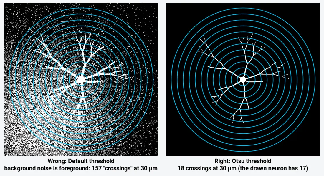
Look at the mask before counting. Triangle, Otsu and Li all gave the same clean profile on this image, within one crossing; Default and Huang did not. On real neurons, also remove other cells' processes that enter the circles: they are counted as branches of yours.
Reading the Sholl plot
- Rising part: branching near the soma. A steep rise means many primary and secondary branches close to the cell body.
- Peak: the maximum and the critical radius. A higher peak means more branches at the busiest distance; a peak further out means branching happens more distally.
- Falling part and tail: where branches end. A long tail with a few crossings (here 4 and 2 crossings at 45 and 50 µm) is one or two long dendrites reaching further than the rest.
- Area under the curve: the sum of crossings, which tracks total dendritic length for a given step. Compare sums only between analyses with the same step.
To compare groups (treated against control neurons), compare the whole profiles, for example with a two-way repeated-measures ANOVA or a mixed model on radius × group, as well as the summary numbers; a difference in the peak alone can hide a shift in where the branches are.
Pitfalls
- A noisy mask. Background specks count as crossings. Check the overlay; the threshold comparison above shows how badly it can go.
- Neighbouring neurons. Their processes crossing your circles add to your counts. Crop, clear outside or erase them first.
- A centre off the soma. Shifting the centre changes every radius. Use the soma's centre (the thickest point), and the same rule for every cell.
- Comparing sums across different steps. The sum and mean scale with the number of circles.
- 2D projections of 3D neurons. A maximum-intensity projection merges branches that cross in depth and shortens those that run along Z. Analyse the stack in 3D (Fiji) when the arbor is thick.
- The step too coarse. With 20 µm steps you can miss the peak. Use 1–5 µm for cultured neurons.
- Uncalibrated images. Radii in pixels cannot be compared between microscopes. Set the scale first.
Reporting it
A methods sentence to copy, with the parts in brackets filled in:
Dendritic complexity was quantified by Sholl analysis (Sholl, 1953) in [Fiji/SNT (Ferreira et al., 2014) / ImageJ 1.54f with a custom macro]. Neurons were thresholded ([Otsu]) and isolated, the centre was placed on the soma, and crossings were counted on circles from [5] to [60] µm in [5] µm steps. We report the maximum number of crossings, the critical radius and the ramification index (maximum ÷ number of primary dendrites) for [n] neurons from [N] cultures.
Show the profile as mean ± SEM per radius for each group, with one example neuron and its circles.
Next: measure neurite length and branching with a skeleton.
An easier way: Sholl analysis online in LabCanvas
LabCanvas Image Analysis has Sholl analysis as a guided assay in the browser: no Fiji, no update site, no macro to paste.
- Open the image (a TIFF with its µm scale, or set the scale) and choose Assays › Sholl analysis.
- The cell is found with a threshold; the centre is the Cell body, found automatically as the thickest point, or Click on the image to place it.
- Count on the Cell or its Skeleton, and set the radii: From, To (auto reaches the farthest tip) and Every (2 µm in the screenshot).
- Click Count intersections: the circles, crossings and centre are drawn on the image, with the Sholl plot beside them.
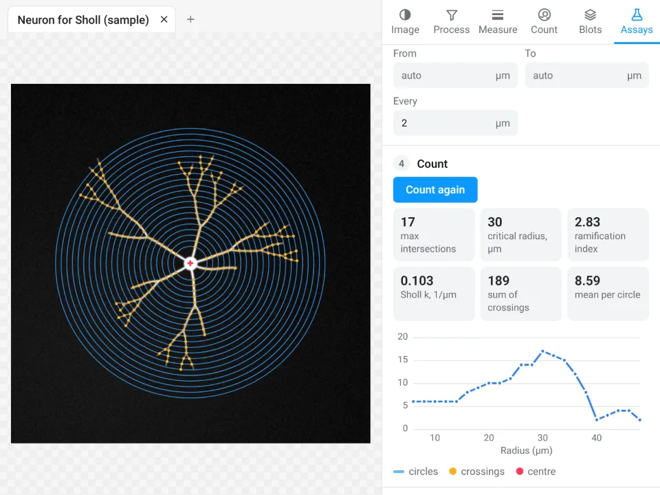
On the same synthetic neuron LabCanvas finds a maximum of 17 crossings at 30 µm and a ramification index of 2.83 (
Why it is a good choice for Sholl analysis:
- Nothing to install and no plugin to update: it runs in the browser on any computer or tablet.
- The summary numbers Fiji reports: maximum, critical radius, ramification index, sum and mean, primary branches and the regression coefficient k with its R².
- The table and profile go straight to Graphs for the profile plot, with a methods sentence to copy; free with a LabCanvas account (CSV download is part of Pro), and every measurement is checked in more than 4,000 automated tests.
Use Fiji's SNT instead for 3D (spheres through a stack), traced reconstructions (SWC files), polynomial fits of the profile, or a macro over hundreds of neurons. Open Image Analysis.
ImageJ and Fiji are independent open-source projects; LabCanvas is not affiliated with them.
References
- Sholl DA (1953). Dendritic organization in the neurons of the visual and motor cortices of the cat. Journal of Anatomy 87, 387–406. PMID 13117757, PMC1244622
- Ferreira TA, Blackman AV, Oyrer J, Jayabal S, Chung AJ, Watt AJ, Sjöström PJ, van Meyel DJ (2014). Neuronal morphometry directly from bitmap images. Nature Methods 11, 982–984. doi:10.1038/nmeth.3125
- Arshadi C, Günther U, Eddison M, Harrington KIS, Ferreira TA (2021). SNT: a unifying toolbox for quantification of neuronal anatomy. Nature Methods 18, 374–377. doi:10.1038/s41592-021-01105-7
- Schindelin J, Arganda-Carreras I, Frise E, et al. (2012). Fiji: an open-source platform for biological-image analysis. Nature Methods 9, 676–682. doi:10.1038/nmeth.2019
Frequently asked questions
What is Sholl analysis?
Sholl analysis counts how many times a neuron's branches cross a series of concentric circles (or spheres in 3D) centred on the cell body. Plotted against the radius, the counts show how dendritic complexity changes with distance from the soma. Sholl introduced the method in 1953.
How do I do Sholl analysis in Fiji?
Threshold the neuron so the arbor is foreground, mark the centre (a point on the cell body, or a straight line from the soma outwards), and run the Sholl Analysis command that comes with SNT in Fiji. Set the starting radius, ending radius and step size; it returns the crossings per radius, the plot and the summary metrics. Type "Sholl" in Fiji's search bar to find the command in your version.
Can I do Sholl analysis in plain ImageJ without plugins?
Yes, with a short macro. Threshold and convert the neuron to a mask, put a point on the cell body, and count background-to-foreground transitions along each circle. The macro on this page does that and draws the circles; on our sample it gives a peak of 18 crossings at 30 µm.
What is the ramification index in Sholl analysis?
The Schoenen ramification index is the maximum number of crossings divided by the number of primary branches leaving the cell body. A neuron with 6 primary dendrites and at most 17 crossings has a ramification index of
What is the critical radius?
The critical radius is the distance from the centre at which the number of crossings is largest; the number of crossings there is the critical value or maximum. On our sample the ImageJ macro puts it at 30 µm, where the drawn neuron has its maximum too.
Can I do Sholl analysis online?
Yes. LabCanvas Image Analysis has a Sholl assay in the browser (Assays › Sholl analysis) that finds the cell body, counts the crossings and reports the maximum, critical radius, ramification index and Sholl regression coefficient.
Try it in LabCanvas
Every app is free to start in your browser. Create an account and begin.
Start Image Analysis free in your browserKeep reading
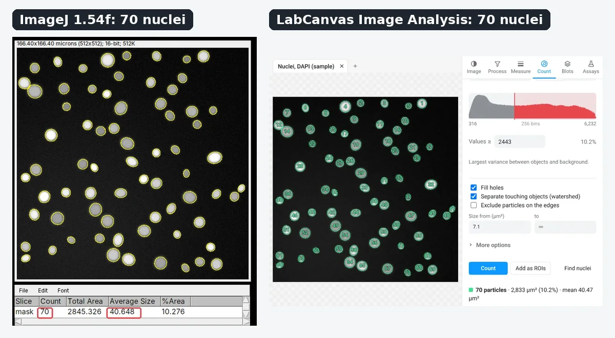
ImageJ vs LabCanvas Image Analysis: an honest comparison
ImageJ/Fiji or LabCanvas Image Analysis? Six everyday jobs done in both, six newer ones (macros, vendor files, 3D, StarDist, big images) and which to use.
How to use ImageJ: a beginner's tutorial for the 10 everyday jobs (2026)
How to use ImageJ and Fiji: get started, open an image, then 10 everyday jobs (scale, measure, threshold, count, background, blots) with exact menu paths.
How to set the scale and add a scale bar in ImageJ (with a calibration image to practise on)
Set the scale in ImageJ (Analyze › Set Scale) from a micrometer, scale bar or pixel size, add a scale bar, and practise on a free calibration image.