Plot Profile in ImageJ: line scans, wide lines and intensity profiles
Plot Profile in ImageJ: draw a line, press Ctrl K, set the line width to average noise, copy the values, plot two channels and profile a rectangle.
Contents
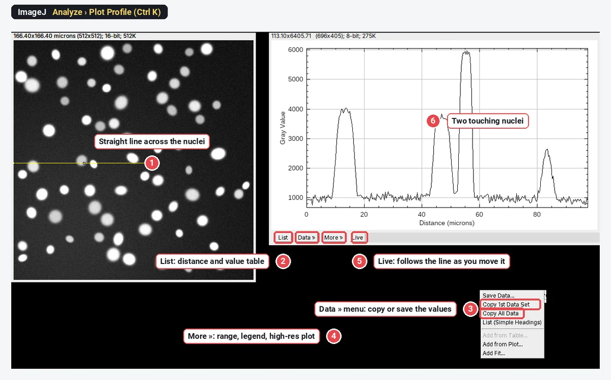
To plot an intensity profile in ImageJ, draw a line across the structure with a line tool and choose Analyze › Plot Profile (Ctrl K): a window plots the pixel values against distance along the line, in µm if the image is calibrated. Click List for the numbers, Data » to copy or save them, and Live to make the plot follow the line as you move it; set a wider line (double-click the line tool) to average noise across it.
A line profile, or line scan, is the simplest quantitative look at an image: the values along one path, nothing more. Below: the plot window explained, line width with a real example, profiles of two channels, profiles of a rectangle, and the other profile tools in ImageJ. Every picture is ImageJ 1.54f on our synthetic sample images, not real lab data.
How do I plot a line profile in ImageJ (or Fiji)?
Plot Profile is part of ImageJ 1.x, so these steps are the same in Fiji.
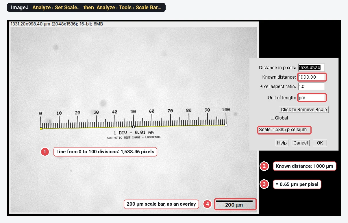
- Open the image. Check the scale with Image › Properties…: with a pixel size the x-axis reads in µm, without it in pixels.
- Pick a line tool in the toolbar: Straight, Segmented (click points, double-click to finish) or Freehand. Right-click the tool to switch between them.
- Draw the line across what you want to scan. Zoom in first if the ends matter; one pixel is a lot on a small structure.
- Analyze › Plot Profile, or Ctrl K. The plot opens in its own window.
- Read or export the values with the buttons under the plot.
What do List, Data, More and Live do?
| Button | What it does |
|---|---|
| List | Opens a table of Distance and Gray Value, one row per point along the line |
| Data » | Save Data… (a CSV file), Copy 1st Data Set, Copy All Data, List (Simple Headings), Add from Table…, Add from Plot…, Add Fit… |
| More » | Set Range…, Reset Range, Set Range to Fit All, Zoom to Selection, Axis Options…, Legend…, Contents Style…, High-Resolution Plot…, Freeze Plot, Plot Defaults… and a few more |
| Live | The plot redraws whenever you move the line, drag an end or change the slice or channel |
Two of these save time every day. Live turns placing a line scan into a few seconds of nudging the line until the peak is centred. Set Range… fixes the axes, so plots from several images can be compared by eye; set it once for all profiles in a figure.
The number of points equals the length of the line in pixels: a 300-pixel line gives about 300 values, spaced one pixel apart. Values between pixel centres are interpolated (the Interpolate box in Edit › Options › Plots…, ticked by default).
How do I set the line width, and why does it matter?
A one-pixel line samples one pixel at each point, so every bit of noise shows. A wider line averages the pixels across its width at each point along it. The signal along the line stays; the noise shrinks roughly with the square root of the width.
To set it:
- Double-click the line tool in the toolbar. That opens Image › Adjust › Line Width, a small window with a slider.
- Or Edit › Options › Line Width… and type the width in pixels.
- For a line already drawn, press y (Edit › Selection › Properties) and change its width there.
A wide line shows on the image as a band, so you can see exactly which pixels are averaged.
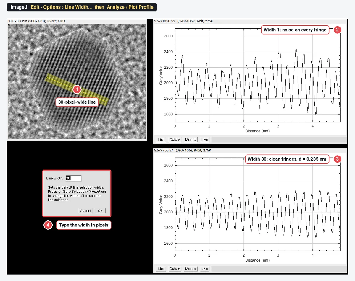
That example is a real measurement in miniature. On the 30-pixel profile we found the peaks with ImageJ's Array.findMaxima: the first at 0.22 nm and the last at 4.68 nm along the line, 19 spacings apart, so the lattice spacing is
How wide? As wide as the structure stays straight and uniform across the line. On fringes, the line must run exactly across them: a tilted wide line averages neighbouring fringes into each other and flattens the peaks. On a cell edge or a membrane, a width of 3 to 10 pixels is typical; on a filament, keep the width close to the filament's own width or you average in background.
How do I plot a profile of two channels?
Analyze › Plot Profile in ImageJ 1.54f plots only the channel that is selected in a multichannel image. To compare channels you have two options:
- Step through the channels with Live on. Move the channel slider; the plot redraws for each channel, one at a time.
- Plot both in one graph with a short macro. It reads the profile of each channel along the current line and draws them together:
Stack.setChannel(1); p1 = getProfile();
Stack.setChannel(2); p2 = getProfile();
getPixelSize(unit, pw, ph);
x = newArray(p1.length);
for (i = 0; i < x.length; i++) x[i] = i * pw;
Plot.create("Both channels", "Distance (" + unit + ")", "Gray value");
Plot.setColor("green"); Plot.add("line", x, p1);
Plot.setColor("magenta"); Plot.add("line", x, p2);
Plot.setLegend("Channel 1\tChannel 2", "top-right");
Plot.show();
Run it with Plugins › New › Macro, paste, and Run. It respects the line width you set.
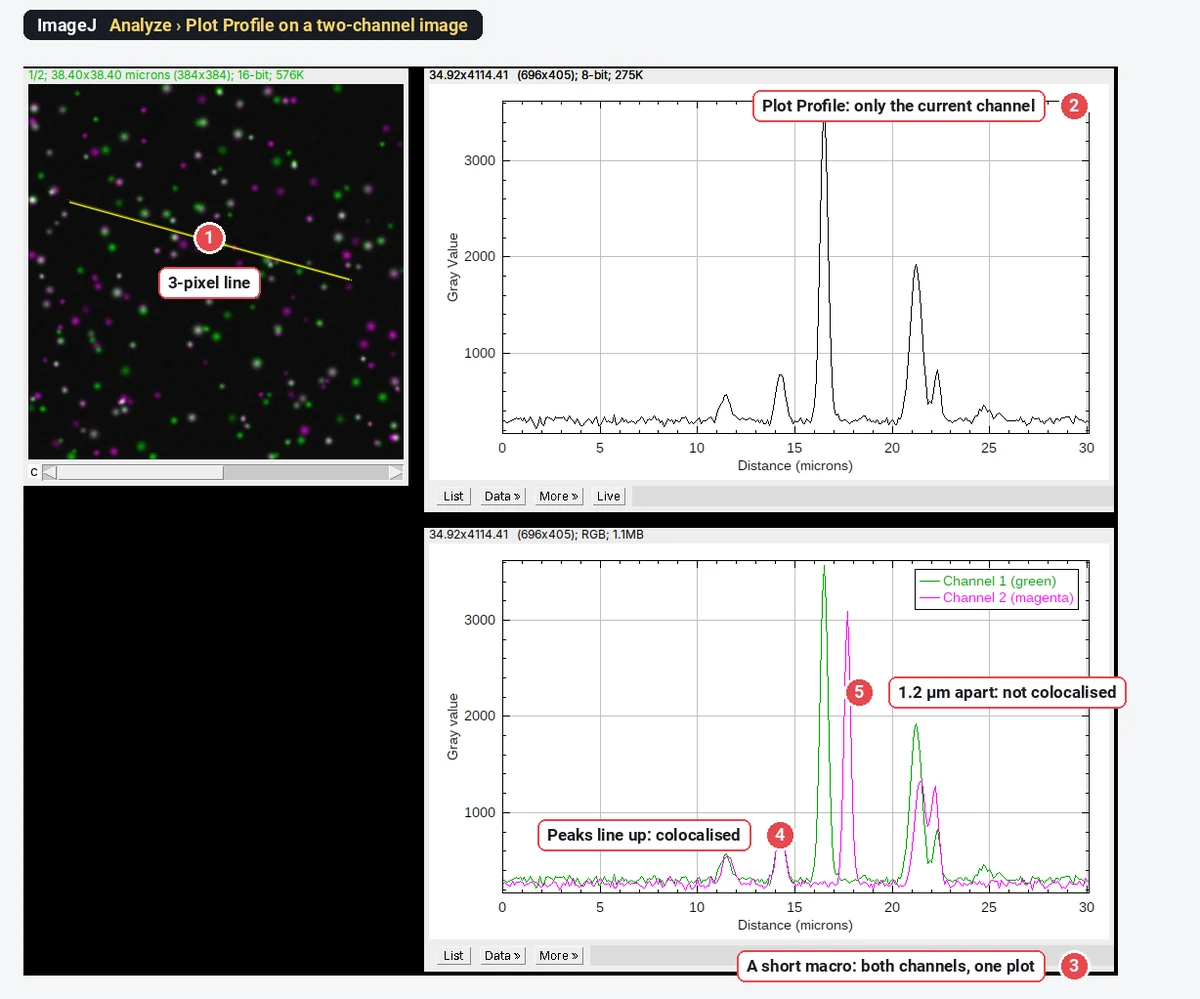
A two-channel line scan is a good way to show colocalisation in a figure: peaks that coincide, and peaks that do not, are easy to read. It is not a colocalisation measurement. A line samples a few hundred pixels picked by hand, so it can show whatever you choose to show. For numbers, use Pearson's and Manders' coefficients over the whole cell (see colocalisation analysis), and use the line scan to illustrate them.
The channels must be aligned for any of this to mean anything. A chromatic shift of 1 or 2 pixels between channels moves every peak; check it on multicolour beads before you trust a 100 nm offset.
What does Plot Profile do with a rectangle?
Draw a rectangle instead of a line and Plot Profile gives a column average: each point along the x-axis is the mean of one column of the rectangle. A long, thin rectangle across a row of bands or cells is in effect a very wide line, with every pixel in it used.
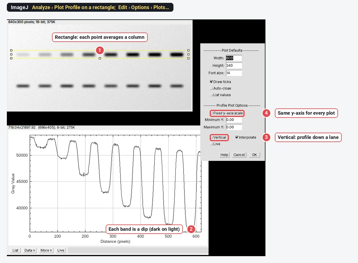
For a profile that runs down the rectangle (a row average, for example along one lane of a gel), either hold Alt as you press K, or tick Vertical under Profile Plot Options in Edit › Options › Plots…. The same dialog has Fixed y-axis scale with a Minimum and Maximum Y, which keeps every profile on the same axis; that matters when you show profiles side by side.
On a blot, remember that bands are dark: lower values mean more protein. ImageJ's Analyze › Gels commands handle lanes and band areas for you; see western blot quantification.
Other profile tools in ImageJ
- Segmented and freehand lines follow a curved structure (an axon, a cell edge); the x-axis is the distance along the path. Combined with a time-lapse and Image › Stacks › Reslice, that is a kymograph.
- Image › Stacks › Plot Z-axis Profile plots the mean of a selection through the slices or frames of a stack: a time course, or intensity against depth.
- ROI Manager › More » › Multi Plot plots the profiles of several line selections stored in the ROI Manager on one graph.
- Analyze › Surface Plot shows the whole image as a 3D landscape, the same idea in two dimensions.
Pitfalls
- An uncalibrated image. The x-axis reads in pixels. Set the scale first (Analyze › Set Scale…).
- A one-pixel line on noisy data. Peaks and widths come out ragged. Widen the line, along the structure, not across a gradient.
- A wide line across a curved or tilted structure blurs it. Keep the band perpendicular to edges and fringes.
- Saturated pixels. A flat-topped peak at the maximum value (255, 4095 or 65535) is clipped; its true height is unknown.
- Comparing profiles with auto-scaled axes. Fix the y-range (More » › Set Range… or Fixed y-axis scale).
- Measuring on an RGB or flattened copy. Profile the raw image, not the version with an overlay burnt in.
- One hand-picked line as evidence. Report how lines were placed, and show several.
Reporting it
A methods sentence to copy:
Line intensity profiles were measured in [Fiji (ImageJ 1.54f)] with Analyze › Plot Profile along [straight] lines [3] pixels ([0.3] µm) wide, drawn [perpendicular to the membrane through the centre of each cell]; values were exported and plotted in [software].
Show profiles with fixed axes, give the line width in the legend, and mark the line on the image panel. Cite ImageJ or Fiji.
An easier way: line profiles in LabCanvas
The same line scan works in the browser, with nothing to install, in LabCanvas Image Analysis, and a multichannel image needs no macro.
- Click Open an image (a TIFF keeps its scale and channels), or the two-channel sample on the start screen.
- Pick the Line tool (L) and draw across the structure.
- Open Measure › Profile: the plot is live as you draw and move the line, with one curve per channel. Set Line width to average across the line; hovering over the plot marks the point on the image.
- Add to results for the numbers, then Copy table, or Send to Graphs with the XY option for a figure-ready profile.
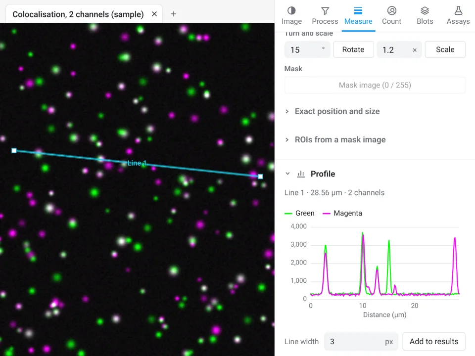
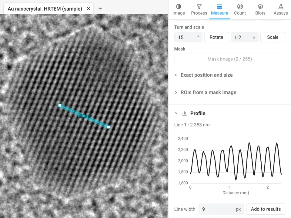
On the HRTEM gold sample, the Profile panel finds 10 spacings over 2.353 nm, d = 0.235 nm; ImageJ's 30-pixel profile above gave the same 0.235 nm from 19 spacings over 4.46 nm.
Why it is a good choice for line scans:
- Nothing to install: it runs in the browser on any computer or tablet.
- Every channel at once, from the raw values, with no macro.
- Straight into Graphs: the XY profile becomes a plot with axis labels and styling, and the table carries a methods sentence to copy.
- Free with a LabCanvas account; downloading the CSV is part of LabCanvas Pro. The measurements are checked in more than 4,000 automated tests.
ImageJ and Fiji are stronger when you need hundreds of profiles placed by a macro, or profiles on files in a maker's format that only Bio-Formats reads. Open Image Analysis and try a line scan on the two-channel sample. ImageJ and Fiji are independent open-source projects; LabCanvas is not affiliated with them.
References
- Schneider CA, Rasband WS, Eliceiri KW (2012). NIH Image to ImageJ: 25 years of image analysis. Nature Methods 9, 671–675. doi:10.1038/nmeth.2089
- Schindelin J, Arganda-Carreras I, Frise E, et al. (2012). Fiji: an open-source platform for biological-image analysis. Nature Methods 9, 676–682. doi:10.1038/nmeth.2019
Frequently asked questions
How do I plot an intensity profile in ImageJ?
Draw a line with the Straight, Segmented or Freehand line tool, then choose Analyze › Plot Profile (Ctrl K). A plot window opens with distance along the line on the x-axis (in calibrated units if the image has a scale) and the pixel values on the y-axis. Click List for the numbers.
How do I make a wider line for Plot Profile?
Double-click the line tool in the toolbar (it opens Image › Adjust › Line Width) or use Edit › Options › Line Width…, and type a width in pixels. Plot Profile then averages the pixels across that width at each point along the line, which smooths noise. Press y (Edit › Selection › Properties) to change the width of a line you have already drawn.
How do I copy the Plot Profile values to Excel?
In the plot window, click Data » and choose Copy 1st Data Set (or Copy All Data), then paste. Or click List to open a table of distance and value and copy from there; Data » Save Data… writes a CSV file.
Can ImageJ plot a profile of several channels at once?
Not with Analyze › Plot Profile in ImageJ 1.54f: it plots the channel that is selected. Step the channel slider with Live on, or run a short macro that reads getProfile() for each channel and adds them to one plot (shown on this page).
What does Plot Profile do with a rectangle?
It plots a column average: each point is the mean of one column of the rectangle, so a wide rectangle averages a lot of noise away. For a row average (a profile running down the rectangle), hold Alt as you press K, or tick Vertical in Edit › Options › Plots….
What is the Live button in the plot window?
With Live on, the plot follows the selection: move the line or its ends, or change the slice or channel, and the profile redraws. It is the quickest way to place a line scan across a structure.
Try it in LabCanvas
Every app is free to start in your browser. Create an account and begin.
Start Image Analysis free in your browserKeep reading
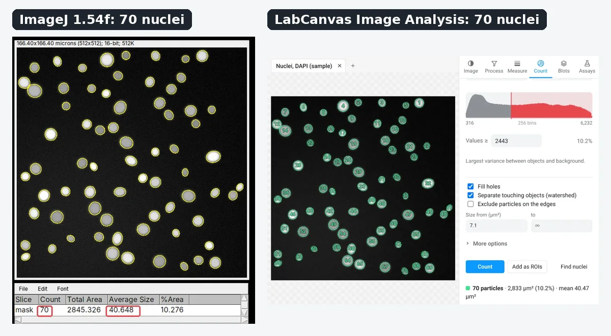
ImageJ vs LabCanvas Image Analysis: an honest comparison
ImageJ/Fiji or LabCanvas Image Analysis? Six everyday jobs done in both, six newer ones (macros, vendor files, 3D, StarDist, big images) and which to use.
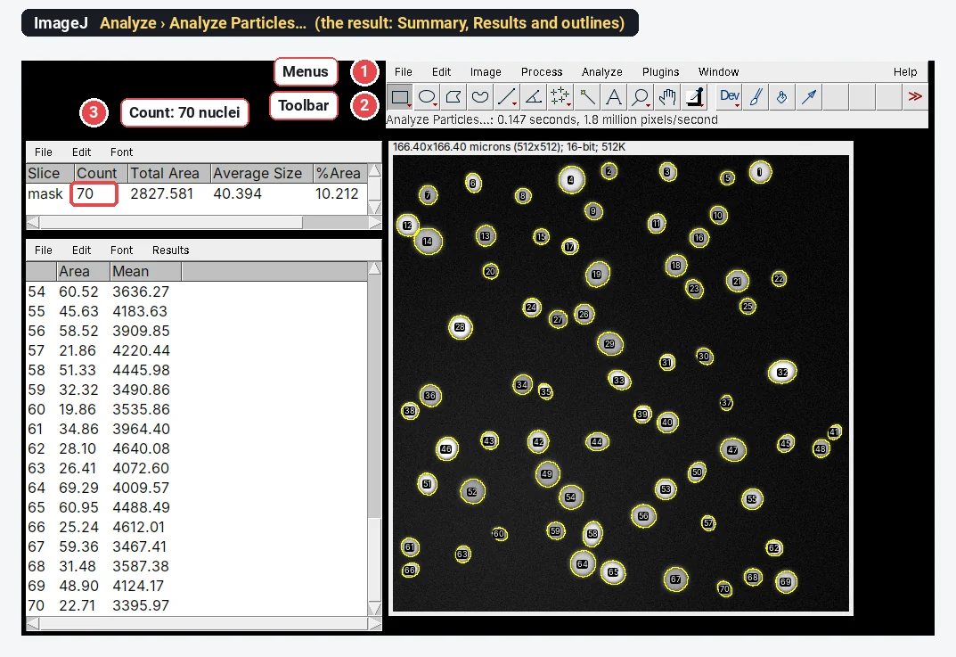
How to use ImageJ: a beginner's tutorial for the 10 everyday jobs (2026)
How to use ImageJ and Fiji: get started, open an image, then 10 everyday jobs (scale, measure, threshold, count, background, blots) with exact menu paths.
How to set the scale and add a scale bar in ImageJ (with a calibration image to practise on)
Set the scale in ImageJ (Analyze › Set Scale) from a micrometer, scale bar or pixel size, add a scale bar, and practise on a free calibration image.