Colocalization analysis in ImageJ: Pearson vs Manders and Costes thresholds
Colocalization in ImageJ and Fiji: what Pearson’s r and Manders’ M1/M2 each answer, Costes thresholds, Coloc 2 vs JACoP, a worked example and pitfalls.
Contents
Plain ImageJ 1.x has no colocalisation command: use Coloc 2 in Fiji (Analyze › Colocalization › Coloc 2) or the JACoP plugin. Both report Pearson's r, which asks whether the two channels' intensities rise and fall together, and Manders' M1 and M2, which ask what fraction of each channel's signal lies where the other channel has signal. Costes thresholds decide automatically which pixels count as signal; without them, Manders' coefficients are close to meaningless.
On the synthetic two-channel sample used below, Pearson's r is 0.529 and Manders above the Costes thresholds is about 0.22 for each channel.
Pearson vs Manders: which coefficient answers which question?
| Coefficient | Question it answers | Range | Depends on thresholds? |
|---|---|---|---|
| Pearson's r | Do the two intensities vary together, pixel by pixel? | −1 to 1 | No (all pixels); "r above thresholds" uses only signal pixels |
| Manders M1 | What fraction of channel 1's intensity sits where channel 2 is present? | 0 to 1 | Yes, entirely |
| Manders M2 | What fraction of channel 2's intensity sits where channel 1 is present? | 0 to 1 | Yes, entirely |
| tM1, tM2 | M1 and M2 with "present" defined by the Costes thresholds | 0 to 1 | Costes |
| Spearman's ρ | Like Pearson, on ranks, so a few very bright pixels sway it less | −1 to 1 | No |
| Overlap coefficient | Manders' 1993 overlap, | 0 to 1 | No, but strongly affected by background |
| Li's ICQ | Do the channels tend to be above or below their means together? | −0.5 to 0.5 | No |
The formulas, with
Pearson's
Pick by your question. "Does protein X go where Y goes?" is Manders M1 (the share of X found on Y). "Does Y go where X goes?" is M2, and the answer can be different: a protein that sits only on mitochondria has an M1 near 1 against a mitochondrial marker, while most of the marker (M2) can be far from it. "Do X and Y vary together, so that more X means more Y?" is Pearson. Report both kinds; they answer different questions.
How to do colocalisation in Fiji with Coloc 2
- Open the two-channel image. If the channels are separate files, keep them as they are; Coloc 2 takes two images.
- Draw an ROI around one cell (or make a binary mask of the cells), so that empty background is not counted.
- Run Coloc 2 (Analyze › Colocalization › Coloc 2; press L and type "Coloc 2" if the menu reads differently in your version).
- Choose Channel 1 and Channel 2, the ROI or mask, and Threshold regression: Costes.
- Tick what you want reported (Li's ICQ, Spearman, Manders, Kendall's tau, 2D histogram, Costes significance test). For the significance test, set the PSF size in pixels (about the size of the smallest spot) and the number of randomisations (more is slower but steadier).
- Click OK. Coloc 2 shows a PDF-like report with the 2D histogram, the thresholds, Pearson's r below and above them, tM1 and tM2, and the P-value of the Costes test.
Coloc 2 comes with Fiji; it is not part of plain ImageJ 1.x.
JACoP (Just Another Colocalization Plugin)
JACoP, by Bolte and Cordelières (2006), predates Coloc 2 and is still widely cited. It is a separate plugin: in Fiji, enable the update site that provides it (the BIOP version is distributed through the PTBIOP update site) or drop the JACoP .jar in the plugins folder of ImageJ. Choose the two images, tick the coefficients (Pearson, Overlap, k1/k2, Manders with thresholds, Costes' automatic threshold and randomisation, Van Steensel's CCF, Li's ICQ, object-based methods) and adjust the threshold of each channel on its preview.
JACoP's object-based option (centres of mass and distances between objects) is something pixel-based tools such as Coloc 2 do not give, and it suits punctate stains.
What plain ImageJ 1.x can show you
Without a plugin, ImageJ 1.x still lets you look at the two channels together and compute the basic numbers.
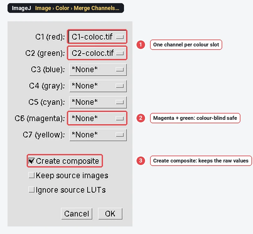
See the overlap. Image › Color › Merge Channels… puts two single-channel images into one composite. Give one channel the green slot and the other the magenta slot (not red, which reads poorly for colour-blind viewers), and keep Create composite ticked so the original 16-bit values stay in separate channels. White then marks the overlap. Image › Color › Channels Tool… switches channels on and off.
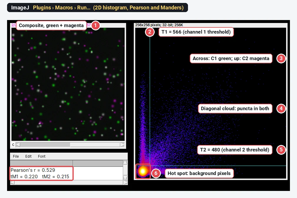
Compute Pearson and thresholded Manders. This macro (Plugins › Macros › Run…, or paste it into Plugins › New › Macro and click Run) splits the active two-channel image, computes Pearson's r over all pixels, Manders' tM1 and tM2 for the thresholds you type in, and draws a 2D histogram (a scatter plot of channel 1 against channel 2, with the number of pixels at each pair of values shown in colour) with the thresholds as cyan lines. It works on the whole image; crop to one cell first (Image › Crop) to analyse a cell.
// Pearson's r, thresholded Manders and a 2D histogram for a two-channel image (plain ImageJ 1.x)
T1 = 566; T2 = 480;   // thresholds for channel 1 and 2: Costes values from Coloc 2, or your own
title = getTitle();
run("Split Channels");
selectImage("C1-" + title); w = getWidth(); h = getHeight(); n = w * h;
x = newArray(n); for (j = 0; j < h; j++) for (i = 0; i < w; i++) x[j*w + i] = getPixel(i, j);
selectImage("C2-" + title);
y = newArray(n); for (j = 0; j < h; j++) for (i = 0; i < w; i++) y[j*w + i] = getPixel(i, j);
Array.getStatistics(x, min1, max1, m1); Array.getStatistics(y, min2, max2, m2);
sxy = 0; sxx = 0; syy = 0; s1 = 0; s2 = 0; c1 = 0; c2 = 0;
for (k = 0; k < n; k++) {
  dx = x[k] - m1; dy = y[k] - m2; sxy += dx*dy; sxx += dx*dx; syy += dy*dy;
  s1 += x[k]; s2 += y[k];
  if (y[k] >= T2) c1 += x[k];
  if (x[k] >= T1) c2 += y[k];
}
print("Pearson's r = " + d2s(sxy / sqrt(sxx * syy), 3));
print("tM1 = " + d2s(c1 / s1, 3) + "   tM2 = " + d2s(c2 / s2, 3));
// 2D histogram: channel 1 across, channel 2 up, 256 x 256 bins, log of the counts
b = 256; newImage("2D histogram", "32-bit black", b, b, 1);
for (k = 0; k < n; k++) {
  i = floor(x[k] / (max1 + 1) * b); j = b - 1 - floor(y[k] / (max2 + 1) * b);
  setPixel(i, j, getPixel(i, j) + 1);
}
run("Add...", "value=1"); run("Log"); run("Fire"); resetMinAndMax();
makeLine(T1 / (max1 + 1) * b, 0, T1 / (max1 + 1) * b, b); Overlay.addSelection("cyan");
makeLine(0, b - T2 / (max2 + 1) * b, b, b - T2 / (max2 + 1) * b); Overlay.addSelection("cyan");
run("Select None");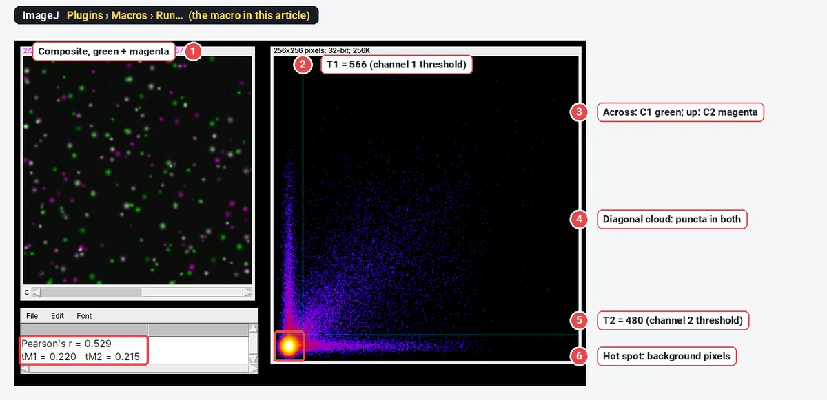
How to read a 2D histogram: points along the diagonal are pixels bright in both channels (colocalised and correlated); points along one axis are bright in that channel only; the dense spot near the origin is background. A tight diagonal cloud gives a high Pearson's r; two arms along the axes pull it down.
Worked example: one image, three thresholds
The sample is synthetic: 160 green puncta, about 60% of which have a magenta partner at the same place, on a background of about 310 (channel 1) and 270 (channel 2), the median of each channel. Pearson's r over all pixels, from the ImageJ macro, is 0.529.
Manders' coefficients on the same image, computed by the macro with three different thresholds:
| Thresholds (channel 1, channel 2) | M1 | M2 | Pixels above both |
|---|---|---|---|
| None (0, 0) | 1.000 | 1.000 | 147,456 (every pixel) |
| Costes (566, 480) | 0.220 | 0.215 | 7,193 |
| Otsu on each channel (1223, 1061) | 0.135 | 0.135 | 2,922 |
Without thresholds, every pixel has some signal in the other channel because of the camera offset, so
How do Costes thresholds work?
Costes et al. (2004) fit a straight line through the 2D histogram (an orthogonal regression of channel 2 on channel 1). They then start with the thresholds at the top of that line and lower them step by step, each time computing Pearson's r of the pixels below either threshold. When that r reaches zero or below, the pixels below the thresholds show no correlation: they are taken as background, and the pixels above both thresholds are the signal. For this sample the line ends at about 566 for channel 1 and 480 for channel 2.
Costes also proposed a significance test: shuffle one channel in blocks the size of the point-spread function many times, recompute r each time, and see how often a random image correlates as well as the real one. If the real r beats nearly all randomisations (P > 0.95 in Coloc 2's convention), the colocalisation is unlikely to be chance.
Costes thresholds fail when the channels are barely correlated or the background is very uneven; Coloc 2 then warns that the regression did not give sensible thresholds. Check the 2D histogram before trusting them.
Pitfalls in colocalisation analysis
- Background. A camera offset or diffuse background inflates unthresholded Manders and the overlap coefficient, and an uneven background can create correlation where there is none. Use thresholds (Costes, or set on a single-stained control) and an ROI around the cells.
- Bleed-through (crosstalk). If the green dye shows up in the red channel, you will measure colocalisation that is pure optics. Image single-stained controls with the same settings: any signal in the "empty" channel is bleed-through. Use sequential scanning on a confocal and well-separated dyes.
- Chromatic shift. The two colours may not focus at exactly the same place, shifting one channel by a pixel or more. Image multicolour beads and correct the shift before measuring.
- The ROI. A whole field with empty background and many cells gives a different r from one cell. Measure per cell (draw an ROI or use a mask), and say which you did.
- Saturation and processing. Saturated pixels cut off the top of the 2D histogram and lower r; 8-bit or RGB conversion rescales each channel differently. Measure the raw files; deconvolution, if you use it, must be applied the same way to every image.
- Resolution. Colocalisation at the light-microscope limit (about 200 nm laterally, more in z) means "within the same resolution volume", not binding. Proving an interaction takes FRET, a proximity ligation assay or super-resolution.
- A random control. Rotate one channel by 90° (Image › Transform › Rotate 90 Degrees Right) and measure again: r should drop to around 0. If it does not, something other than the biology (background, bleed-through, cell shape) is driving the number.
Reporting it
A methods sentence to copy, with the parts in brackets filled in:
Colocalisation was analysed in [Fiji (ImageJ 1.54f) with Coloc 2] on [single confocal sections / maximum projections] acquired sequentially with identical settings. For each cell, an ROI was drawn around the cell; Pearson's correlation coefficient and Manders' coefficients (tM1, tM2) were calculated above automatic Costes thresholds (Costes et al. 2004), and significance was assessed with the Costes randomisation test ([PSF] pixels, [100] randomisations). [n] cells from [3] independent experiments were analysed per condition.
Name the software and plugin, the coefficient (Pearson, tM1 or M1) and how thresholds were set. Show the values per cell as a dot plot with the replicate means highlighted, and include a representative merged image with the single channels beside it, in magenta and green, with a scale bar.
An easier way: colocalisation in LabCanvas
If you would rather not install Fiji or paste a macro, LabCanvas Image Analysis calculates the same coefficients in the browser, with the definitions of Coloc 2 and nothing to install.
- Open your two-channel image (or the Two channels sample on the start screen) and go to Measure › Colocalisation.
- Choose the two channels and the region: the selected ROI or the whole image.
- Set the thresholds to Costes (auto) and click Calculate.
- Tick Show colocalised to mark the pixels above both thresholds in yellow on the image.
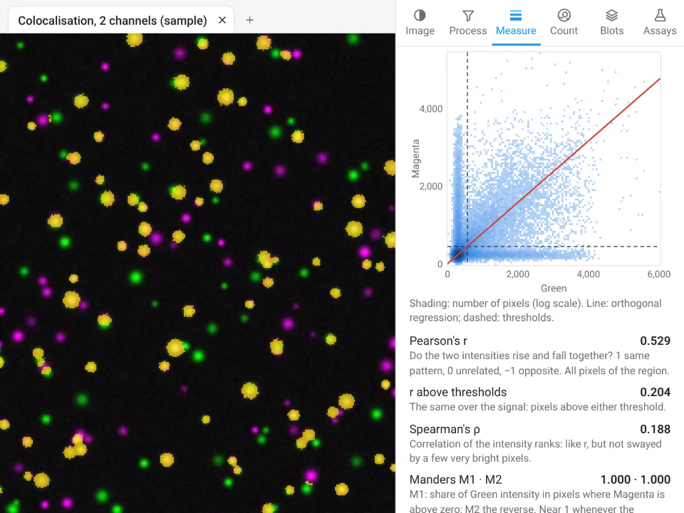
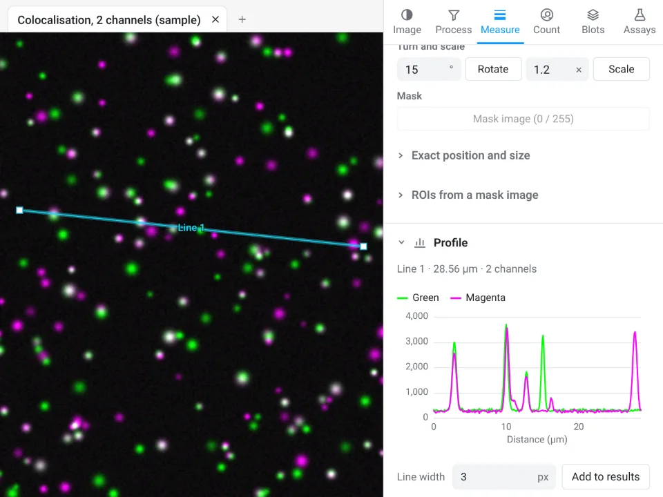
On the same synthetic sample, LabCanvas gives Pearson's r 0.529 (the ImageJ macro: 0.529) and tM1 0.219 and tM2 0.214 above the Costes thresholds, with 7,169 colocalised pixels (the macro: 0.220, 0.215 and 7,193). The third decimal differs only because of where the threshold search stops.
Why it is a good choice for colocalisation:
- Nothing to install and no macro: Pearson's r, r above the thresholds, Spearman's ρ, M1 and M2, tM1 and tM2, the overlap coefficient and Li's ICQ in one table, each with a one-line explanation.
- Checks before you calculate: Process › Align › Channels measures and corrects a shift between the channels, and the image check flags clipped pixels.
- Straight into Graphs: Send to Graphs turns the per-cell values into a graph with statistics, and the table carries a methods sentence to copy.
- Free with a LabCanvas account (downloading CSV files is part of LabCanvas Pro), and every measurement is checked in more than 4,000 automated tests.
Fiji is still the choice for object-based colocalisation (JACoP), the Costes randomisation test with a PSF model, 3D object analysis and batch scripts over many images. Open Image Analysis, or read the complete guide.
ImageJ and Fiji are independent open-source projects; LabCanvas is not affiliated with them.
References
- Bolte S, Cordelières FP (2006). A guided tour into subcellular colocalization analysis in light microscopy. Journal of Microscopy 224, 213–232. doi:10.1111/j.1365-2818.2006.01706.x
- Costes SV, Daelemans D, Cho EH, Dobbin Z, Pavlakis G, Lockett S (2004). Automatic and quantitative measurement of protein-protein colocalization in live cells. Biophysical Journal 86, 3993–4003. doi:10.1529/biophysj.103.038422
- Manders EMM, Verbeek FJ, Aten JA (1993). Measurement of co-localization of objects in dual-colour confocal images. Journal of Microscopy 169, 375–382. doi:10.1111/j.1365-2818.1993.tb03313.x
- Schindelin J, Arganda-Carreras I, Frise E, et al. (2012). Fiji: an open-source platform for biological-image analysis. Nature Methods 9, 676–682. doi:10.1038/nmeth.2019
Frequently asked questions
How do I do colocalization analysis in ImageJ?
Plain ImageJ 1.x has no colocalisation command. Use Fiji, which ships Coloc 2 (in the Analyze › Colocalization menu): choose the two channels, an optional ROI or mask, Costes threshold regression, and it reports Pearson’s r, Manders’ M1 and M2 above the Costes thresholds and a 2D histogram. JACoP is an older plugin that does much the same and is installed separately.
What is the difference between Pearson and Manders coefficients?
Pearson’s r asks whether the two intensities rise and fall together across the pixels (from −1 to 1). Manders’ M1 and M2 ask what fraction of each channel’s signal sits where the other channel has signal (from 0 to 1), and the two can differ: M1 can be high while M2 is low. Pearson is about correlation, Manders about overlap.
What are Costes thresholds?
Costes et al. (2004) set a threshold for each channel automatically: fit a line through the 2D histogram, then lower the two thresholds along that line until the pixels below them show no correlation (Pearson’s r ≤ 0). Pixels above both thresholds count as signal. Manders’ coefficients computed with these thresholds are called tM1 and tM2.
Why are my Manders coefficients 1.0?
Because no threshold was applied and the background is not zero. Unthresholded Manders counts every pixel where the other channel is above 0, and with a camera offset that is every pixel. Use Costes thresholds or thresholds set on a control.
Is JACoP or Coloc 2 better?
Both give Pearson, Manders and Costes. Coloc 2 is maintained, ships with Fiji, works on ROIs and masks and adds the Costes significance test; JACoP (Bolte and Cordelières 2006) adds object-based colocalisation and Van Steensel’s and Li’s methods. Whichever you use, name it and its settings in the methods, because their thresholded Manders definitions are not always identical.
What Pearson value means colocalisation?
There is no universal cut-off. r close to 1 means the intensities vary together, around 0 means no relation, below 0 means they avoid each other. Compare r between conditions measured the same way, and with a control such as one channel rotated 90°, rather than reading a single value against a fixed threshold.
Try it in LabCanvas
Every app is free to start in your browser. Create an account and begin.
Start Image Analysis free in your browserKeep reading
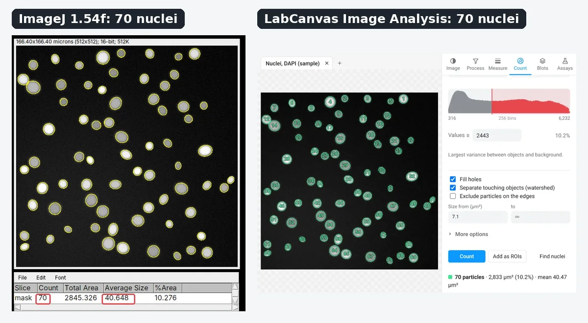
ImageJ vs LabCanvas Image Analysis: an honest comparison
ImageJ/Fiji or LabCanvas Image Analysis? Six everyday jobs done in both, six newer ones (macros, vendor files, 3D, StarDist, big images) and which to use.
How to use ImageJ: a beginner's tutorial for the 10 everyday jobs (2026)
How to use ImageJ and Fiji: get started, open an image, then 10 everyday jobs (scale, measure, threshold, count, background, blots) with exact menu paths.
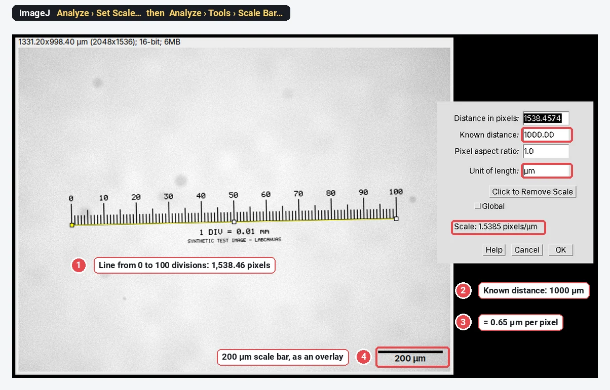
How to set the scale and add a scale bar in ImageJ (with a calibration image to practise on)
Set the scale in ImageJ (Analyze › Set Scale) from a micrometer, scale bar or pixel size, add a scale bar, and practise on a free calibration image.