Western blot quantification in ImageJ, step by step (and the 3-click way)
Quantify a western blot in ImageJ with Analyze › Gels, normalise to a loading control or total protein, and get fold change. Plus a 3-click way.
Contents
To quantify a western blot in ImageJ, draw a rectangle over each lane with Analyze › Gels › Select First Lane and Select Next Lane, plot the lanes with Plot Lanes, close each band's peak with a straight line and click inside it with the Wand to get its area. Then divide each target band by the loading control (or the total protein) in the same lane, and divide that ratio by the one in your control lane:
Below are the full ImageJ steps with a worked example on a blot whose answer is known, the mistakes that make blot numbers wrong, and a methods sentence to copy.
Before you start: quantify the right file
The numbers can only be as good as the image you measure.
- Use the original file from the imager: the TIFF it saves (usually 16-bit), not a JPEG, a screenshot or a copy adjusted for a figure.
- Check that no band is saturated. A saturated band has hit the top of the detector's range, so its area is too small, and no software can get the lost signal back (see Pitfalls).
- Film: scan it in greyscale, at a fixed setting, with any automatic contrast correction switched off.
- Straight lanes: if the blot is tilted, rotate it first with Image › Transform › Rotate….
In ImageJ (or Fiji): Analyze › Gels, step by step
The gel analyser is part of ImageJ 1.x, so it is the same in plain ImageJ and in Fiji. Its commands sit in Analyze › Gels: Select First Lane (keyboard shortcut 1), Select Next Lane (2), Plot Lanes (3), Re-plot Lanes, Reset, Label Peaks and Gel Analyzer Options.
1. Check the options
Open Analyze › Gels › Gel Analyzer Options… once before you start:
| Option | Default | What it does |
|---|---|---|
| Invert peaks | On | Inverts the values so that dark bands become upward peaks. Keep it on for dark bands on a light background; turn it off for light bands on a dark background (fluorescent blots, stain-free images). |
| Label with percentages | On | Label Peaks writes each peak as a percentage of all the peaks you measured, instead of its area. |
| Uncalibrated OD | Off | Converts the values to uncalibrated optical density, a log scale meant for scanned film. It works on 8-bit values, so a 16-bit image is converted to 8-bit first. Leave it off for a digital imager's file. |
| Vertical and horizontal scale factor | 1 | The size of the lane plots on screen. It does not change the ratios. |
2. Select the lanes
- Pick the Rectangle tool and draw a box over the first lane: a little narrower than the band, and tall enough to take in background above and below it.
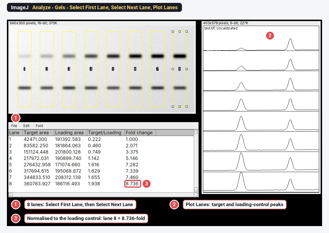
- Choose Analyze › Gels › Select First Lane. ImageJ takes the lanes to be vertical unless the box is at least twice as wide as it is tall; then it asks whether the lanes are horizontal.
- Drag the same box (click inside it and drag) onto lane 2 and choose Analyze › Gels › Select Next Lane. Repeat for every lane. Don't resize the box: ImageJ refuses with "Selections must all be the same size", and for vertical lanes it keeps every box level with the first.
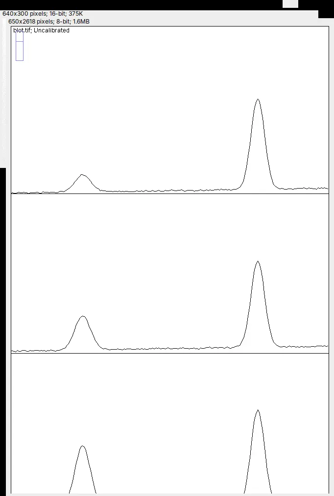
- Choose Analyze › Gels › Plot Lanes. A window opens with one profile per lane, stacked top to bottom, and ImageJ switches to the straight-line tool for the next step.
3. Close off each peak
Each band is a peak in its lane's profile. With the straight-line tool, draw a line across the foot of each peak, from the background level on its left to the background level on its right, so that the peak becomes a closed area. Where two bands run into each other, also draw a line from the dip between them down to that baseline. These lines are your background subtraction, so place them the same way in every lane.
4. Read the peak areas with the Wand
- Pick the Wand tool and click inside each closed peak, in lane order. Each click adds a row with its Area to the Results table (nothing is measured while Shift is held down).
- Choose Analyze › Gels › Label Peaks. Each peak is labelled on the plot with its share of the total, and the Results table now lists Area and Percent for every peak.
- Copy the table into a spreadsheet before you measure anything else: the first Wand click on the next plot starts a new table.
5. Measure the loading control or the total protein
Repeat steps 2 to 4 for the loading-control band (β-actin, GAPDH, tubulin) with its own boxes, and copy its table too.
For total-protein normalisation, open the image of the stained membrane (Ponceau S, Coomassie, a stain-free gel) and set Invert peaks to match it: Ponceau S and Coomassie are dark on light, stain-free images are light on dark. Use boxes that cover the whole length of each lane, close each lane's profile with one line from end to end, and click it with the Wand: that area is the lane's total protein.
6. Normalise in the spreadsheet
Each Plot Lanes window is scaled to its own range, so a target area and a loading-control area taken from two different plots are not on the same scale. Compare lanes within each plot first, then divide:
| Quantity | How to get it |
|---|---|
| Relative density of the target | the target's Percent (or Area) in the lane ÷ the same in the control lane |
| Relative density of the loading control | the loading control's Percent in the lane ÷ the same in the control lane |
| Normalised density (fold change) | relative density of the target ÷ relative density of the loading control |
The control lane comes out at 1, and a lane with twice as much target per unit of protein comes out at 2. Run at least three independent blots and compare their fold changes with a statistical test; one blot is an anecdote.
Worked example: a blot with a known answer
The sample is a synthetic 16-bit blot made from known amounts: eight lanes, a target band that rises across them, and a loading control with small lane-to-lane differences, as on a real blot. The true fold change of lane 8 is 8.935. In ImageJ 1.54f each band's area was integrated above a straight baseline between the background on either side, the rule the line-and-wand steps follow (done here by a short macro so that every band is closed the same way), then divided as in step 6.
| Lane | 1 | 2 | 3 | 4 | 5 | 6 | 7 | 8 |
|---|---|---|---|---|---|---|---|---|
| Target ÷ loading control | 0.222 | 0.460 | 0.749 | 1.142 | 1.616 | 1.629 | 1.655 | 1.938 |
| Fold change | 1.000 | 2.071 | 3.375 | 5.146 | 7.282 | 7.339 | 7.460 | 8.736 |
Lane 2 shows why the loading control matters: its target band alone is 1.97 times lane 1's, but its loading control is a little weaker, so the fold change is 2.071. Lane 8 at 8.736-fold is within 2.5% of the true 8.935; the small shortfall comes from where the baselines sit and how much of each band's tails falls inside the box, so place them the same way in every lane and every blot.
Pitfalls
Saturated bands and the linear range
A band is saturated when its brightest pixels reached the limit of the detector, so they all sit at the top value (65,535 in a full-range 16-bit file), or at 0 in a file that shows dark bands on light. Its peak in the lane plot has a flat top and its area is too small, so the strongest bands are underestimated and real differences shrink. In ImageJ, point at the band and read the value in the status bar, or tick Min & max gray value in Analyze › Set Measurements… and measure a box around it; Analyze › Histogram shows a spike at the top value when many pixels are clipped. The fix is at acquisition: a shorter exposure, guided by the imager's own saturation warning.
Not saturated is not enough. The signal also has to be in the linear range, where twice the protein gives twice the signal. Check it once for each antibody with a two-fold dilution series of a pooled sample on the same blot (Taylor et al. 2013; Pillai-Kastoori et al. 2020). On one blot, Taylor and colleagues found film linear over a 16-fold range of their target protein against 128-fold for a camera imager, and GAPDH linear only up to about 0.5 µg of cell lysate, far below the 10 to 50 µg most labs load. Abundant loading controls such as β-actin and GAPDH are often overloaded in this way (Aldridge et al. 2008), and skipping these checks can make blots overestimate or underestimate real differences (Janes 2015).
Background: the choice changes the answer
Gassmann et al. (2009) applied several common densitometry procedures to the same western blot and got p values ranging from 0.000013 to 0.76 for the same correlation. Choose one method, use it for every lane and every blot, and report it.
- In the gel analyser, the line closing each peak is the background. Its ends must sit on background on both sides, not on the shoulder of a neighbouring band.
- For a sloping or blotchy background, flatten it first with Process › Subtract Background… (tick Light background for dark bands) and a radius larger than the bands; see rolling-ball background subtraction.
- If you measure a box around each band with Analyze › Measure instead, the background inside the box is counted too: subtract the same-sized box from an empty area next to the band.
Lane width and placement
- Keep the box narrower than the band, so that no lane takes in the gap between lanes. The lane profile is the mean across the box's width, so a box that strays onto empty membrane lowers the band.
- Use the same width for every lane. ImageJ enforces it.
- For a smiling or tilted gel, rotate the image or make the boxes tall enough, and check in Plot Lanes that each peak sits at the same place in every lane.
Uneven loading, and what a loading control must do
Normalising corrects unequal loading only if the loading control is itself measured in its linear range and does not change with your treatment. Look at its raw areas: if they swing with the condition rather than with how much you loaded, it is not a loading control for this experiment.
Why many journals prefer total-protein normalisation
A total-protein stain (Ponceau S, Coomassie, Amido Black, SYPRO Ruby or a stain-free gel) measures all the protein in the lane, not one abundant protein that may saturate or respond to the treatment. Aldridge et al. (2008) found that GAPDH and β-actin did not accurately reflect differences in loading at the protein amounts used for less abundant targets, and that the total-protein stains SYPRO Ruby and Amido Black were acceptable alternatives. Gilda and Gomes (2013) found stain-free total-protein staining a better loading control than β-actin, and as good as or better than Ponceau S. Pillai-Kastoori et al. (2020) set out the whole validation workflow, from linear range to normalisation.
JPEGs, screenshots and adjusted images
JPEG compression changes pixel values, contrast and gamma changes alter the ratios between bands, and a screenshot is an 8-bit picture of the screen, not the data. Quantify the original file and adjust a copy for the figure; Image › Type should say 16-bit (or 8-bit) for an imager's file, and Image › Show Info… shows where it came from. See image integrity for microscopy and blots for what you may and may not do to a blot image.
Reporting it
A methods sentence to copy, with the parts in brackets filled in:
Western blots were imaged on [imager] and quantified by densitometry in [ImageJ 1.54 (Analyze › Gels)] on the unadjusted [16-bit TIFF] files. Lanes were defined with rectangles of equal width, and each band's area was integrated above a straight baseline drawn between the background on either side of the band. No band was saturated. Target bands were normalised to [total protein (Ponceau S) / β-actin] in the same lane and expressed as fold change relative to [the control lane]. Data are mean ± SD of [n = 3] independent blots.
Cite ImageJ (Schneider et al. 2012; see how to cite ImageJ and Fiji), and give the box width, the background method and what you normalised to.
To show the result, plot the fold change for each condition with every blot as a point and the mean ± SD, name the test, and put a representative blot next to it. Keep the uncropped original images: journals often ask for them.
ImageJ is the better choice if you run the same analysis on hundreds of blots with a macro, or need a plugin for an unusual workflow. For the other free options, see free western blot quantification software.
The 3-click way: quantify the blot in LabCanvas
LabCanvas Image Analysis does the same measurement in the browser, on the raw 8- or 16-bit values, with no lane boxes to drag and no spreadsheet. Open the blot's TIFF (or the built-in western blot sample, the same synthetic blot as above) and go to the Blots tab.
- Lanes: Find lanes finds them from the image, all the same width (or draw rectangles and click Use selected).
- Bands: Find bands proposes a window for each band row; name them, mark the loading control, and tick Align lanes if the gel smiles.
- Quantify: choose the Background (Straight line, as in ImageJ, Rolling or None), what to Normalise to (the loading-control band or a Total protein stain image) and the Reference lane.
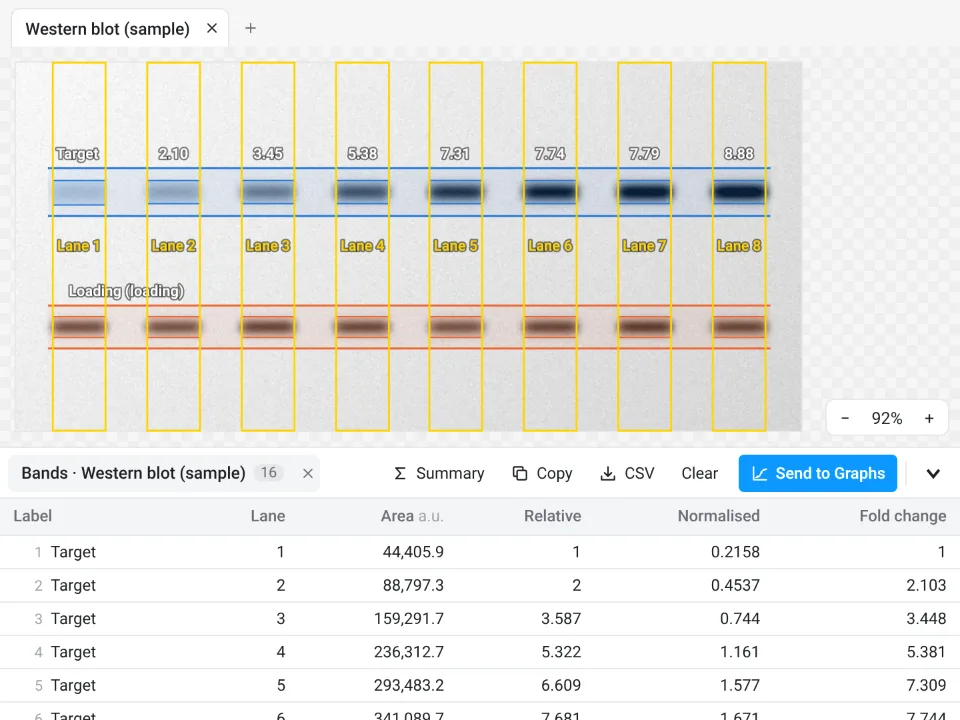
On the same blot, LabCanvas gives lane 2 at 2.103-fold and lane 8 at 8.885-fold, against 2.071 and 8.736 in ImageJ and a true 8.935. The two differ by where each baseline sits and how wide each band window is.
Why it is a good choice for blots:
- One scale for every band: target and loading-control areas come from the same image and scale, so they divide directly, with no separate Plot Lanes windows to reconcile.
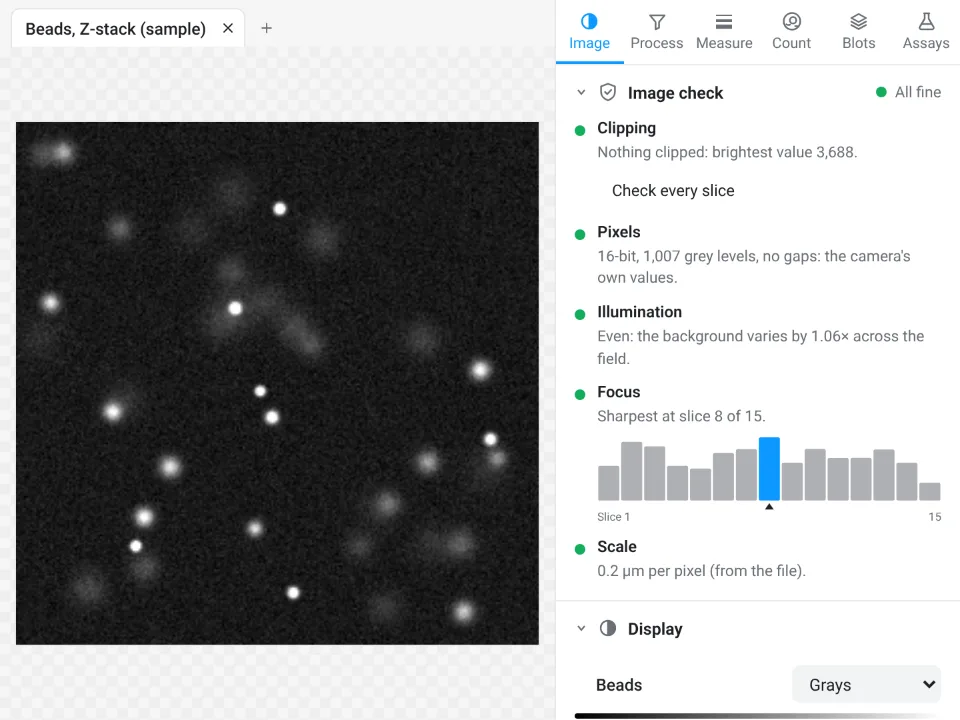
- An image check first: it counts clipped pixels (a saturated band shows up there) and flags JPEGs and pixels taken from a figure.
- Fold change straight into Graphs: the Bands table gives Area, Relative, Normalised and Fold change, Send to Graphs plots the replicate blots, and a Methods sentence describes exactly how it was measured.
- Free with a LabCanvas account; downloading the table as CSV is part of LabCanvas Pro. Every measurement is checked in more than 4,000 automated tests.
Open Image Analysis and click the western blot sample to try it. ImageJ and Fiji are independent open-source projects; LabCanvas is not affiliated with them.
References
- Aldridge GM, Podrebarac DM, Greenough WT, Weiler IJ (2008). The use of total protein stains as loading controls: an alternative to high-abundance single-protein controls in semi-quantitative immunoblotting. Journal of Neuroscience Methods 172, 250–254. doi:10.1016/j.jneumeth.2008.05.003
- Gassmann M, Grenacher B, Rohde B, Vogel J (2009). Quantifying Western blots: pitfalls of densitometry. Electrophoresis 30, 1845–1855. doi:10.1002/elps.200800720
- Gilda JE, Gomes AV (2013). Stain-Free total protein staining is a superior loading control to β-actin for Western blots. Analytical Biochemistry 440, 186–188. doi:10.1016/j.ab.2013.05.027
- Janes KA (2015). An analysis of critical factors for quantitative immunoblotting. Science Signaling 8, rs2. doi:10.1126/scisignal.2005966
- Pillai-Kastoori L, Schutz-Geschwender AR, Harford JA (2020). A systematic approach to quantitative Western blot analysis. Analytical Biochemistry 593, 113608. doi:10.1016/j.ab.2020.113608
- Schneider CA, Rasband WS, Eliceiri KW (2012). NIH Image to ImageJ: 25 years of image analysis. Nature Methods 9, 671–675. doi:10.1038/nmeth.2089
- Taylor SC, Berkelman T, Yadav G, Hammond M (2013). A defined methodology for reliable quantification of Western blot data. Molecular Biotechnology 55, 217–226. doi:10.1007/s12033-013-9672-6
Frequently asked questions
How do I quantify a western blot in ImageJ?
Open the original TIFF from the imager. Draw a rectangle on the first lane and choose Analyze › Gels › Select First Lane, move the same rectangle to each other lane and choose Select Next Lane, then Plot Lanes. Close each band's peak with the straight-line tool, click inside it with the Wand to get its area, and use Label Peaks for percentages. Do the same for the loading control, then divide the target by the loading control and set the control lane to 1.
How do I normalise western blot bands to a loading control?
For each lane, divide the target band's density by the loading-control band's density in the same lane, then divide every lane's ratio by the control lane's ratio, so the control comes out at 1 (the fold change). In ImageJ, work from relative densities (each lane divided by the control lane within one lane plot), because separate Plot Lanes windows are drawn on different scales. A total-protein stain of the membrane can take the place of the single loading-control band.
What is relative density in western blot analysis?
A band's density divided by the density of the same band in a reference lane, usually the control. With ImageJ's gel analyser it is each lane's Percent (or Area) divided by the control lane's. The target's relative density divided by the loading control's relative density is the normalised density, which is the fold change against the control.
Can I quantify a western blot from a JPEG or a scanned film?
You can, with care. JPEG compression changes pixel values, so use the TIFF your imager saves whenever there is one, and never quantify a figure or a screenshot. Film has a much narrower linear range than a camera imager (16-fold against 128-fold on the same blot in Taylor et al. 2013), so scan it in greyscale with automatic contrast switched off, check that no band is saturated, and use exposures within the linear range.
Should I subtract the background before quantifying bands?
Yes. In ImageJ's gel analyser, the straight line you draw across the foot of each peak is the background. For a sloping or blotchy background you can flatten it first with Process › Subtract Background (tick Light background for dark bands). Use the same method for every lane and every blot, and say which one in your methods: different background choices give different results.
Why does ImageJ say "Selections must all be the same size"?
The gel analyser needs one rectangle size for every lane. Move the rectangle by dragging it from inside, without resizing or redrawing it, between Select Next Lane commands. If the size is wrong, start again with Select First Lane.
Try it in LabCanvas
Every app is free to start in your browser. Create an account and begin.
Start Image Analysis free in your browserKeep reading
ImageJ vs LabCanvas Image Analysis: an honest comparison
ImageJ/Fiji or LabCanvas Image Analysis? Six everyday jobs done in both, six newer ones (macros, vendor files, 3D, StarDist, big images) and which to use.
How to use ImageJ: a beginner's tutorial for the 10 everyday jobs (2026)
How to use ImageJ and Fiji: get started, open an image, then 10 everyday jobs (scale, measure, threshold, count, background, blots) with exact menu paths.
How to set the scale and add a scale bar in ImageJ (with a calibration image to practise on)
Set the scale in ImageJ (Analyze › Set Scale) from a micrometer, scale bar or pixel size, add a scale bar, and practise on a free calibration image.