Measure contact angle from a drop photo in ImageJ

Q: How do I measure contact angle in ImageJ?

Open a side view photo of the drop, pick the Angle tool in the toolbar, click a point on the baseline, then the contact point (where drop, solid and air meet), then a point on the tangent to the drop edge, and press M (Analyze › Measure). The Angle column gives the contact angle. Measure both sides and average them.

Q: What is the spherical-cap formula for contact angle?

If the drop is a spherical cap, θ = 2 arctan(2h/d), where h is the drop height and d the base width. For h = 0.652 mm and d = 1.824 mm, θ = 2 arctan(0.715) = 71.1°. It is accurate only for small drops whose shape is not flattened by gravity.

Q: Is there an ImageJ contact angle plugin?

Yes. DropSnake and LB ADSA, from the Biomedical Imaging Group at EPFL, are free ImageJ plugins (Stalder et al. 2006 and 2010). DropSnake fits a smooth curve to the drop edge and reads the angle at each contact point; LB ADSA fits the Young–Laplace equation to axisymmetric sessile drops and also estimates the surface tension.

Measure contact angle in ImageJ with the Angle tool along the tangent, or from drop height and base width: θ = 2·arctan(2h/d). Worked example, plugins.

By LabCanvas teamPublished 6 November 2026Last updated 6 November 202611 min read

ImageJ measuring the contact angle of a sessile water drop with the Angle tool: lines along the baseline and the tangent at each contact point, and a Results table reading 72.0, 72.0 and 63.6 degrees.

Contents

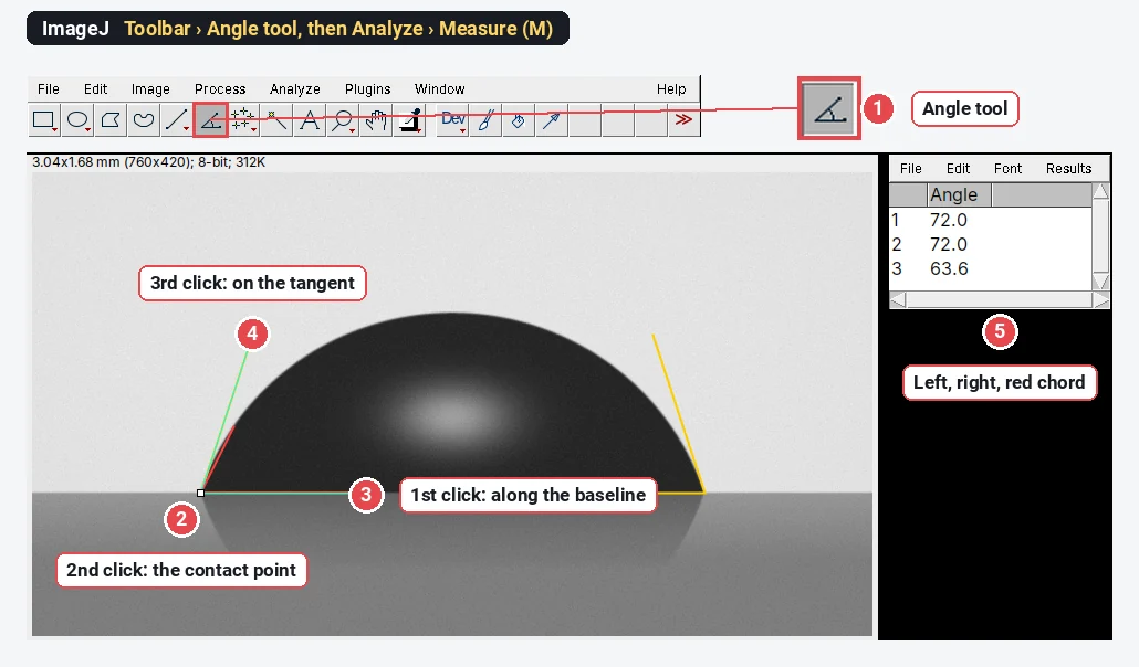
To measure a contact angle in ImageJ, open the side-view drop photo, pick the Angle tool in the toolbar, click once on the baseline, once on the contact point and once along the tangent to the drop edge, then press M (Analyze › Measure): the Angle column is the contact angle. For a small drop you can instead measure its height h and base width d and use the spherical-cap formula, $\theta = 2\arctan(2h/d)$ .

On our test drop, whose true contact angle is 72.0°, the Angle tool read 72.0° on both sides and the spherical-cap formula 71.1°. The rest of this guide shows both methods, where each goes wrong, and the two ImageJ plugins that do it more carefully.

What you are measuring

The contact angle $\theta$ is the angle between the solid surface and the tangent to the liquid surface at the contact point, the place where solid, liquid and air meet, measured through the liquid. Below 90° the liquid wets the surface (hydrophilic for water); above 90° it does not (hydrophobic); above about 150°, superhydrophobic.

The sessile drop method measures it from a side view: a drop sits on the sample, a camera looks at it horizontally, backlit, so the drop is a dark silhouette on a light background with its mirror image in the surface below.

The test image

To check the methods we made a synthetic photo with a known answer: a 1 µL water drop (surface tension 72 mN/m, density 998 kg/m³) with a contact angle of exactly 72°. Its outline is not drawn as a circle: it was computed from the Young–Laplace equation, which includes gravity, as a real drop's would be. It is 760 × 420 pixels at 4 µm per pixel (250 pixels per mm), backlit, with a reflection under the baseline and a little noise. The base is 1.822 mm wide and the drop 0.652 mm high.

Method 1: the Angle tool along the tangent

Open the photo and set the scale if you also want lengths (Analyze › Set Scale…; from the needle's known outer diameter or a calibration target; see how to set the scale in ImageJ). The angle itself needs no scale.
Level the baseline. If the surface is tilted in the picture, rotate the image first (Image › Transform › Rotate…) so that the baseline is horizontal, or simply include the baseline as one arm of the angle, as below, so the tilt cancels.
Zoom in on the left contact point (press + several times, to 400% or more). The contact point is where the drop's silhouette meets its reflection: the narrowest point of the dark "waist".
Pick the Angle tool: it is the toolbar icon with an angle on it, between the line and point tools.
Click three times: first a point on the baseline under the drop, then the contact point (the vertex), then a point on the tangent to the drop edge, just above the contact point. Before the third click, slide the arm until it lies along the last few pixels of the edge.
Press M (Analyze › Measure). The Results table shows the Angle in degrees, between 0 and 180.
Repeat on the right side and report the mean of the two. A difference of more than a few degrees means a tilted stage, a drop that is not symmetrical, or a tangent drawn badly.

The ImageJ Angle tool placed along the baseline and the tangent of a sessile drop, with the Results table — ImageJ 1.54f on the synthetic 1 µL drop true angle 72°. The Angle tool 1, clicked on the baseline 3, at the contact point 2 and along the tangent 4, reads 72.0° on the left and 72.0° on the right. The red line runs to a point 0.24 mm up the edge instead of along the tangent and reads 63.6° 5.

The tangent is where the error lives. The red line in the picture goes from the contact point to a point on the edge only 60 pixels (0.24 mm) higher. That is a chord, not a tangent, and because the edge curves away it reads 63.6°, 8.4° too low. Keep the third click close to the contact point and line the arm up with the very bottom of the edge.

Two practical asides. A drop that is out of focus has a soft edge several pixels wide: focus on the contact line, not on the top of the drop. And the reflection is your friend: the contact point is where the drop and its mirror image meet, which is easier to see than the end of a blurred edge.

Method 2: the spherical-cap formula, θ = 2·arctan(2h/d)

A small drop is close to a slice of a sphere (a spherical cap). For a spherical cap of base width d (twice the base radius) and height h:

\theta = 2\arctan\frac{2h}{d}

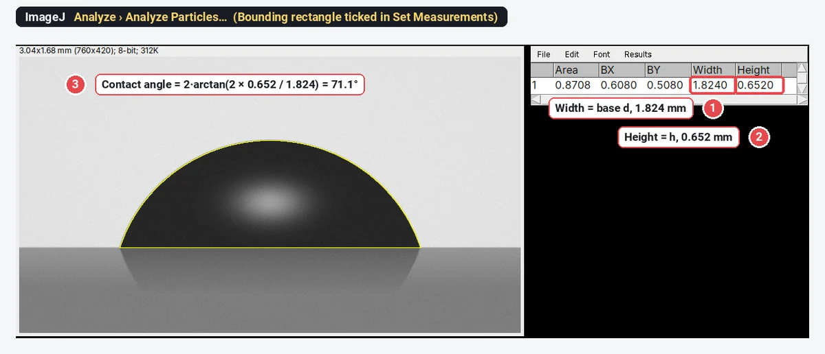
The method needs two lengths instead of a tangent, so it is less sensitive to how you click, but it assumes the shape. Steps in ImageJ:

Set the scale (here 250 pixels = 1 mm).
Draw a rectangle from the top of the image down to the baseline (not past it, or the reflection is included) and duplicate it (Image › Duplicate…).
Image › Adjust › Threshold…, method Default, so that the drop is selected; Apply, then Process › Binary › Fill Holes (the bright highlight in the middle of a backlit drop leaves a hole).
In Analyze › Set Measurements… tick Bounding rectangle, then Analyze › Analyze Particles… with Display results. Width is d and Height is h.

You can also draw two straight lines and press M for each: one between the contact points (d) and one from the apex straight down to the baseline (h).

ImageJ Results table with the width and height of the drop, outlined in yellow — The drop above the baseline thresholded Default, 0–137, holes filled and measured with Analyze Particles: Width 1.824 mm d and Height 0.652 mm h. The spherical-cap formula gives 2·arctan2 × 0.652 / 1.824 = 71.1°.

The worked example

Quantity	Value
Base width d (ImageJ, Width)	1.824 mm (true 1.822 mm)
Height h (ImageJ, Height)	0.652 mm (true 0.652 mm)
$2h/d$	$2 \times 0.652 / 1.824 = 0.715$
$\arctan(0.715)$	35.56°
$\theta = 2 \times 35.56^\circ$	71.1°
True contact angle	72.0°

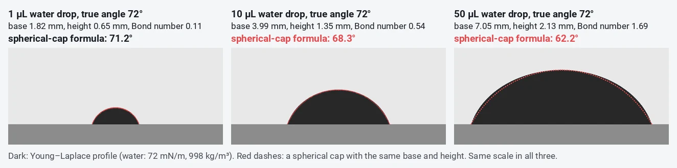
The formula is 0.9° low, and almost all of that is physics, not pixels: even with the exact outline, a 1 µL water drop gives 71.2° by the spherical-cap formula, because gravity has already flattened it slightly.

When does the spherical-cap assumption fail? (Bond number)

Gravity flattens a drop; surface tension rounds it. The Bond number compares the two:

\mathrm{Bo} = \frac{\Delta\rho \, g \, r^2}{\gamma}

where $\Delta\rho$ is the density difference between liquid and air, $g = 9.81\ \mathrm{m/s^2}$ , $r$ the base radius and $\gamma$ the surface tension. When $\mathrm{Bo}$ is much smaller than 1, the drop is close to a spherical cap. The length at which $\mathrm{Bo} = 1$ is the capillary length, $\sqrt{\gamma / \Delta\rho g}$ , 2.7 mm for water at room temperature: drops whose base radius approaches it are visibly flattened.

Three water drops of 1, 10 and 50 µL with the same 72 degree contact angle, and the spherical-cap estimate for each — Three water drops with the same true contact angle, 72°, computed from the Young–Laplace equation and drawn at the same scale, with a spherical cap of the same base and height in red. The spherical-cap formula gives 71.2° at 1 µL Bond number 0.11, 68.3° at 10 µL 0.54 and 62.2° at 50 µL 1.69.

Drop volume (water, true θ 72°)	Base width	Height	Bond number	$2\arctan(2h/d)$	Error
0.5 µL	1.44 mm	0.52 mm	0.07	71.5°	−0.5°
1 µL	1.82 mm	0.65 mm	0.11	71.2°	−0.8°
2 µL	2.30 mm	0.82 mm	0.18	70.7°	−1.3°
5 µL	3.14 mm	1.09 mm	0.34	69.6°	−2.4°
10 µL	3.99 mm	1.35 mm	0.54	68.3°	−3.7°
50 µL	7.05 mm	2.13 mm	1.69	62.2°	−9.8°

Rules of thumb from the table: for the spherical-cap formula, keep water drops at about 1 µL or below (Bond number around 0.1); for the common 2–5 µL drops, use the tangent method or a Young–Laplace fit. Liquids with lower surface tension (oils, ethanol, diiodomethane) flatten more at the same volume. The formula also fails for any drop that is not axisymmetric: on a rough, patterned or chemically patchy surface, or a drop pinned on one side.

The ImageJ contact angle plugins: DropSnake and LB-ADSA

Two free plugins from the Biomedical Imaging Group at EPFL do the fitting for you; download them from the group's Drop Analysis page and put them in the plugins folder of ImageJ or Fiji, then restart.

DropSnake (Stalder et al. 2006) fits a smooth B-spline curve (a "snake") to the drop edge, starting from a few points you click, and reads the angle at each contact point from the fitted curve. It assumes no particular shape, so it also works on drops that are not symmetrical, but it needs a clear edge.
LB-ADSA, low-Bond axisymmetric drop shape analysis (Stalder et al. 2010), fits the Young–Laplace equation (with a first-order correction for gravity) to the whole outline of an axisymmetric sessile drop, and gives the contact angle and an estimate of the surface tension. It suits small, symmetric drops, the same regime as the Bond number table above, and it is less dependent on the few pixels near the contact point.

For routine measurements on many samples, a commercial goniometer with its own Young–Laplace fitting software is faster; the plugins are the free route when you have a camera, a light and a stage.

Taking a good drop photo

Camera level with the surface, looking exactly along it. Tilting the camera down a few degrees shows the top of the surface and moves the apparent contact points.
Backlight through a diffuser behind the drop, so the drop is dark and the edge sharp; no light from the front.
Fill the frame with the drop and a stretch of baseline on both sides, with the edge in sharp focus.
The same volume every time, dispensed gently from a fixed height; note it.
Photograph at a fixed time after deposition (for example 10 s), because drops spread and evaporate. For advancing and receding angles, grow and shrink the drop with the needle in it, or tilt the stage.

Pitfalls

Chord instead of tangent. The most common error, and always in the same direction for a convex drop: too low. On our drop, 63.6° instead of 72.0°.
Wrong contact point. Mistaking the end of the reflection, or the blurred edge, for the contact point shifts the angle by several degrees. Find the waist where drop and reflection meet.
A large drop with the cap formula. At 10 µL of water the formula is already 3.7° low.
Left and right disagree. More than a few degrees apart: level the stage, check that the drop is not pinned, and report both.
Too few drops. Contact angles scatter from drop to drop by a few degrees. Measure at least three to five drops per sample, in different places, and give the mean ± SD.
Static is not the whole story. A single static angle sits somewhere between the advancing and receding angles; their difference (the hysteresis) says how sticky the surface is.

Reporting it

Static water contact angles were measured by the sessile drop method: [2] µL drops of [deionised water] were deposited on the [sample] at [22] °C and photographed from the side after [10] s with a [camera, lens] under diffuse backlighting. Angles were measured in [Fiji (ImageJ 1.54)] with the Angle tool along the tangent at both contact points [or: with the DropSnake plugin], and are given as the mean ± SD of [5] drops on [3] samples.

Cite ImageJ (Schneider et al. 2012) or Fiji (Schindelin et al. 2012), and the plugin you used.

An easier way: contact angle in LabCanvas

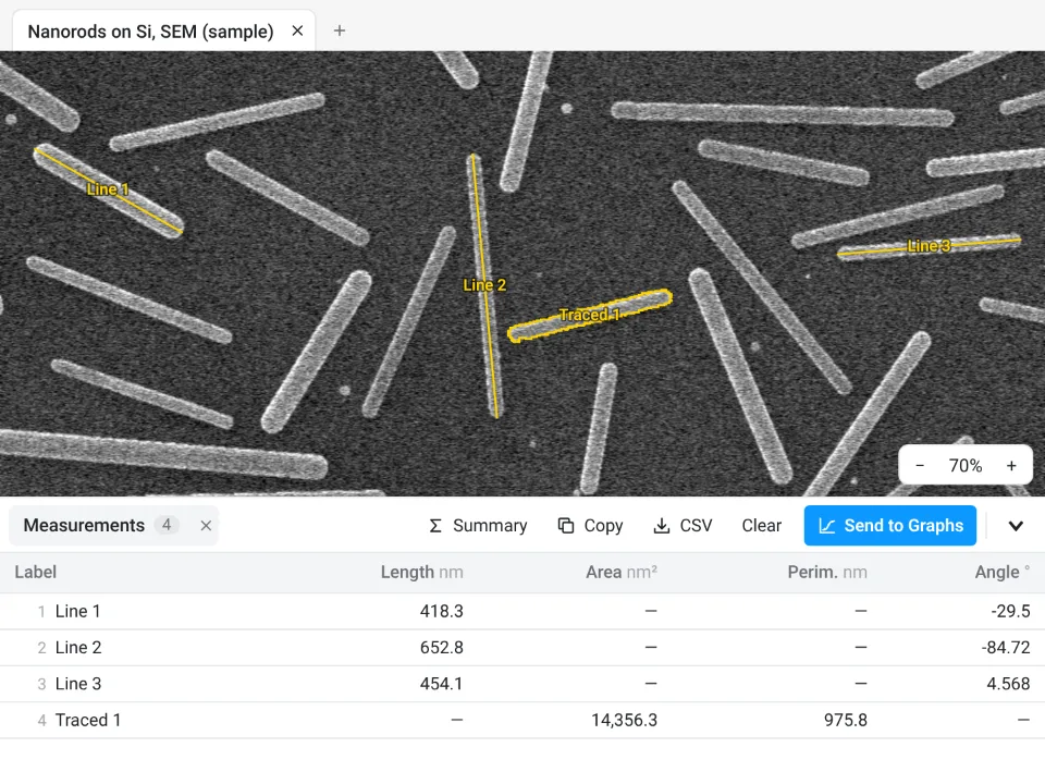
The same two methods work in the browser, with nothing to install, in LabCanvas Image Analysis. It has no dedicated contact-angle tool, but its straight Line tool gives every line a Length and an Angle in the Measurements table, in calibrated units.

Open the drop photo and set the scale in Image › Scale: draw along a known length, type the Known distance and click Set scale.
Tangent method: with the Line tool (L), drag from the left contact point up along the edge and click Measure. The Angle is from the horizontal, so on a level baseline it is the left contact angle; on the right side, drawn the same way, it is 180° minus the contact angle. On a tilted baseline, draw a line along it too and subtract its angle.
Spherical-cap method: draw one line between the contact points (d) and one from the apex down to the baseline (h), select both and Measure; then $\theta = 2\arctan(2h/d)$ .
Send to Graphs to plot the angles by sample or treatment, or Copy the table to a spreadsheet.

Length and area in calibrated units in LabCanvas Image Analysis — The Line tool and Measure in LabCanvas, here on a sample SEM image of nanorods: three lines measured at 418.3, 652.8 and 454.1 nm. On a drop photo the same lines give the base width, the height and, in the Angle column, the angle of the tangent from the horizontal.

Why it is a good choice for drop photos:

Nothing to install: it runs in the browser on any computer or tablet, so you can measure at the goniometer bench.
ImageJ's own names: Length and Angle in the table, and it opens the RoiSet.zip of lines and angles you drew in ImageJ (angles come in as two-segment lines).
Straight into Graphs: Send to Graphs plots the angles by sample without retyping, and Summary adds mean, SD and n rows to the table; each table also carries a methods sentence to copy.
Free with a LabCanvas account: measuring, Copy and Send to Graphs are free; downloading CSV files is part of LabCanvas Pro. The measurements are checked in more than 4,000 automated tests.

LabCanvas does not fit drop shapes: for Young–Laplace fitting or snake-based contact points, use DropSnake or LB-ADSA in ImageJ or Fiji, or a goniometer's software. Open Image Analysis to try it on your own drop photos. ImageJ and Fiji are independent open-source projects; LabCanvas is not affiliated with them.

References

Schindelin J, Arganda-Carreras I, Frise E, et al. (2012). Fiji: an open-source platform for biological-image analysis. Nature Methods 9, 676–682. doi:10.1038/nmeth.2019
Schneider CA, Rasband WS, Eliceiri KW (2012). NIH Image to ImageJ: 25 years of image analysis. Nature Methods 9, 671–675. doi:10.1038/nmeth.2089
Stalder AF, Kulik G, Sage D, Barbieri L, Hoffmann P (2006). A snake-based approach to accurate determination of both contact points and contact angles. Colloids and Surfaces A: Physicochemical and Engineering Aspects 286, 92–103. doi:10.1016/j.colsurfa.2006.03.008
Stalder AF, Melchior T, Müller M, Sage D, Blu T, Unser M (2010). Low-bond axisymmetric drop shape analysis for surface tension and contact angle measurements of sessile drops. Colloids and Surfaces A: Physicochemical and Engineering Aspects 364, 72–81. doi:10.1016/j.colsurfa.2010.04.040

Frequently asked questions

How do I measure contact angle in ImageJ?

Open a side-view photo of the drop, pick the Angle tool in the toolbar, click a point on the baseline, then the contact point (where drop, solid and air meet), then a point on the tangent to the drop edge, and press M (Analyze › Measure). The Angle column gives the contact angle. Measure both sides and average them.

What is the spherical-cap formula for contact angle?

If the drop is a spherical cap, $\theta = 2\arctan(2h/d)$ , where $h$ is the drop height and $d$ the base width. For $h = 0.652\ \mathrm{mm}$ and $d = 1.824\ \mathrm{mm}$ , $\theta = 2\arctan(0.715) = 71.1°$ . It is accurate only for small drops whose shape is not flattened by gravity.

Is there an ImageJ contact angle plugin?

Yes. DropSnake and LB-ADSA, from the Biomedical Imaging Group at EPFL, are free ImageJ plugins (Stalder et al. 2006 and 2010). DropSnake fits a smooth curve to the drop edge and reads the angle at each contact point; LB-ADSA fits the Young–Laplace equation to axisymmetric sessile drops and also estimates the surface tension.

When does the spherical-cap method fail?

When gravity flattens the drop, which depends on the Bond number, $\mathrm{Bo} = \rho g r^2/\gamma$ . For water at 72°, a 1 µL drop (Bo 0.11) gives 71.2° by the cap formula, a 10 µL drop (Bo 0.54) 68.3°, and a 50 µL drop (Bo 1.69) 62.2°. Use drops of about 1 µL or less for the formula, or a tangent or Young–Laplace method for larger ones.

Why do I get a different angle every time I draw the tangent?

The tangent is drawn by eye, right where the edge is blurred by the reflection and the meniscus. Zoom in to 400% or more, find the contact point first, and draw the tangent along the last few pixels of the edge, not to a point further up the drop: on our sample, a line to a point 0.24 mm up the edge read 63.6° instead of 72.0°.

What contact angle means hydrophobic?

By the usual convention, below 90° the surface is hydrophilic (water wets it), above 90° hydrophobic, and above about 150° superhydrophobic. Report the liquid, the drop volume and whether the angle is static, advancing or receding.

contact angle ImageJImageJ contact angle plugindrop analysis ImageJsessile dropDropSnakeLB-ADSAspherical capwettabilityBond numbersurface energy

Try it in LabCanvas

Every app is free to start in your browser. Create an account and begin.

Start Image Analysis free in your browser

Keep reading

The same synthetic nuclei image counted in two programs: on the left ImageJ 1.54f with 70 nuclei outlined in yellow and a Summary of count 70, average size 40.648 µm²; on the right LabCanvas Image Analysis with 70 numbered nuclei and the line 70 particles, mean 40.47 µm²

8 November 202622 min read

ImageJ vs LabCanvas Image Analysis: an honest comparison

ImageJ/Fiji or LabCanvas Image Analysis? Six everyday jobs done in both, six newer ones (macros, vendor files, 3D, StarDist, big images) and which to use.

ImageJ 1.54f with its menu bar and toolbar, a synthetic nuclei image with 70 nuclei outlined and numbered by Analyze Particles, and the Summary and Results tables giving the count, area and mean intensity

6 November 202611 min read

How to use ImageJ: a beginner's tutorial for the 10 everyday jobs (2026)

How to use ImageJ and Fiji: get started, open an image, then 10 everyday jobs (scale, measure, threshold, count, background, blots) with exact menu paths.

ImageJ Set Scale dialog over a synthetic stage micrometer: a line from 0 to 100 divisions measures 1,538.46 pixels, Known distance 1000 µm gives 1.5385 pixels per µm (0.65 µm per pixel), and a 200 µm scale bar sits in the lower right corner as an overlay

6 November 202610 min read

How to set the scale and add a scale bar in ImageJ (with a calibration image to practise on)

Set the scale in ImageJ (Analyze › Set Scale) from a micrometer, scale bar or pixel size, add a scale bar, and practise on a free calibration image.