Grain size analysis in ImageJ (SEM, ASTM E112) + grain size number calculator
Measure grain size from SEM images in ImageJ: closed boundaries, Analyze Particles, then ASTM E112 G from mean area or intercept, with a worked example.
Contents
To measure grain size in ImageJ, set the scale, threshold the image so that every grain is a closed region, and run Analyze › Analyze Particles… with Exclude on edges to get the area of every whole grain. The ASTM E112 grain size number G then follows from the mean grain area
- From the mean area:
- From the mean intercept:
For a nanocrystalline film G comes out above 20, far past the tables in the standard, so report the mean equivalent diameter and its distribution too. The ASTM E112 grain size calculator converts mean area or mean intercept to G and back.
Planimetric or intercept: the two ASTM E112 methods
ASTM E112 (current edition E112-25) describes three ways to estimate the average grain size: comparison with charts, the planimetric (Jeffries) procedure and the intercept (Heyn) procedures. The last two are the ones you can do from an image, and for equiaxed grains they estimate the same G.
| Planimetric (Jeffries) | Intercept (Heyn) | |
|---|---|---|
| What you count | Grains in a known area | Grain boundaries crossed by test lines of known length |
| Counting rule | A grain inside counts 1, a grain cut by the edge ½ | A tangent counts 1, a triple point 1½ |
| What you get | Mean lineal intercept | |
| Best for | Thresholded images and Analyze Particles; it also gives the size distribution | Hand counts, test grids, and images whose boundaries are too faint to segment |
Behind both is the original definition,
In ImageJ (or Fiji)
These steps work in plain ImageJ 1.x unless a step says Fiji. A worked example with real numbers follows.
1. Calibrate and clean the image
- Open the original SEM TIFF, not a screenshot or a JPEG from a slide. Image › Properties… shows whether ImageJ read a pixel size; SEM makers often store it in their own header, which ImageJ may not read.
- Draw a straight line along the scale bar and open Analyze › Set Scale…: type the bar's length in Known distance and nm in Unit of length. Tick Global only if every image you open has the same pixel size.
- Cut off the instrument's data bar: draw a rectangle over the image area and choose Image › Crop, so that the bar is not counted as grains.
- If the file is RGB, convert it with Image › Type › 8-bit.
- Smooth the noise with Process › Filters › Median… at a radius of 1–2 pixels; a median keeps thin boundaries sharper than a Gaussian blur.
- If the brightness drifts across the field (detector position, charging), use Process › Subtract Background… with a rolling ball radius larger than the biggest grain, in pixels. Tick Preview and check that the boundaries do not fade.
2. Threshold so that every boundary stays closed
A grain is only measured correctly if its boundary is a closed line. How you get there depends on how the boundaries look.
Dark boundaries on bright grains (grooved boundaries, as in the sample further down):
- Open Image › Adjust › Threshold…, pick a method (Default, Otsu and MaxEntropy are good first tries) and set it so that the red overlay covers the grains, not the boundaries (the Dark background box flips this).
- Zoom to 200–400% and follow the boundaries: wherever one is broken, two grains will be measured as one. Then click Apply.
- Close a few gaps by hand: a line selection across the gap, then Edit › Draw (it draws in the colour set in Edit › Options › Colors…).
- Use Process › Binary › Watershed only when many boundaries are open. It splits merged round grains, but it also cuts elongated or irregular grains in two; compare the count before and after.
Bright boundaries (secondary-electron images often make boundaries and edges glow):
- Threshold the boundaries themselves, as the bright class, and click Apply: the boundary network is now the foreground.
- Process › Binary › Close- bridges small gaps in the network.
- Process › Binary › Skeletonize thins it to one-pixel lines along the middle of each boundary, so each grain gets its share of the boundary area.
- Process › Binary › Dilate once. Analyze Particles traces 8-connected particles, so two grains could otherwise join through a diagonal step in a one-pixel line.
- Edit › Invert makes the grains the foreground. If Analyze Particles later returns one huge particle, the foreground is the wrong way round: check Process › Binary › Options… › Black background.
When no single threshold separates grains from boundaries, Fiji has two plugins that help: Trainable Weka Segmentation (Plugins › Segmentation › Trainable Weka Segmentation) learns grain and boundary from a few strokes you draw, and MorphoLibJ's Morphological Segmentation (from the IJPB-plugins update site) runs a watershed on the boundary image itself.
3. Measure the grains (planimetric method)
- In Analyze › Set Measurements… tick Area, Shape descriptors, Feret's diameter and Fit ellipse, and Display label.
- Run Analyze › Analyze Particles…: Size (nm^2) from just above the largest speck to Infinity, Circularity 0.00–1.00, Show: Outlines (or Overlay), and tick Display results, Clear results, Summarize, Exclude on edges and Include holes (a pinhole inside a grain stays part of the grain).
- The Summary window gives Count, Total Area and Average Size; Average Size is
- ImageJ has no equivalent-diameter column: compute
- Analyze › Distribution… draws a histogram of any column of the Results table (Area or Feret, for example), with automatic or chosen bins.
- For the strict Jeffries count, run Analyze Particles again with Exclude on edges off: the difference between the two counts is the number of grains cut by the frame, and
Every option in that dialog is explained in Analyze Particles in ImageJ, explained.
4. The intercept method
- Start from a mask of the boundaries thinned to one pixel (step 2, bright-boundary route; for dark boundaries, threshold the boundaries instead of the grains and skeletonise them).
- Overlay test lines with Analyze › Tools › Grid… (ImageJ 1.50f and later): Grid type Lines or Horizontal Lines, with Area per point setting the spacing. The grid is an overlay, so it does not change the pixels.
- Count the crossings with the Multi-point tool: a line tangent to a boundary counts 1, a line through a triple point 1½. For a handful of lines, a quicker check is a straight line selection and Analyze › Plot Profile: each boundary it crosses is a peak.
- Divide the total line length (in calibrated units, converted to mm) by the number of crossings to get
- Count several hundred crossings, spread over several fields, for a stable mean.
Worked example: grain size of a perovskite film in ImageJ
The sample is a top-view SEM image of a perovskite film (synthetic, generated with known grains for these guides): 1024 × 1024 pixels at 2.5 nm per pixel, 8-bit, bright grains with dark grooved boundaries, a few small bright platelets and some pinholes. In ImageJ 1.54f:
- Open the TIFF. The title bar reads 2560x2560 nm, so the scale came with the file; there is no data bar to crop.
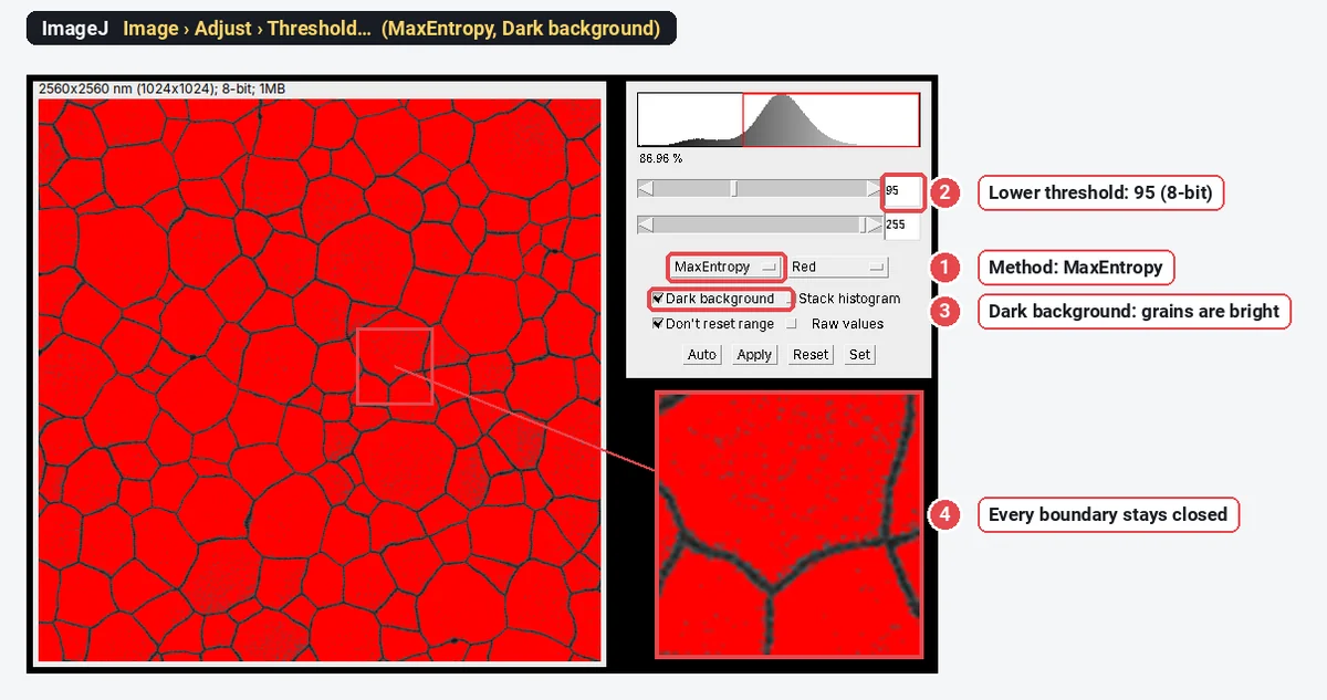
- Image › Adjust › Threshold…: method MaxEntropy, Dark background ticked (the grains are the bright class). The cut falls at 95 and every boundary stays closed, so no watershed is needed.
- Analyze › Set Measurements…: Area and Feret's diameter.
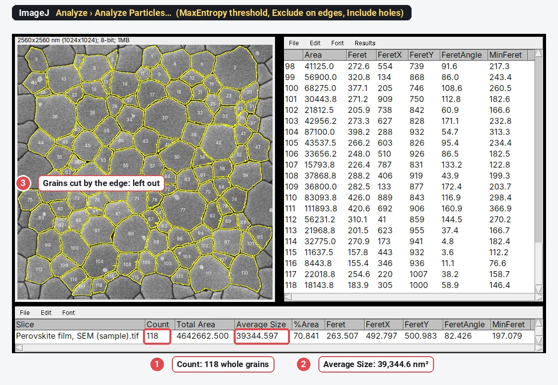
- Analyze › Analyze Particles…: Size 3000-Infinity nm² (to drop the platelets and specks), Display results, Clear results, Summarize, Exclude on edges, Include holes and Overlay.
The result: 118 grains (those cut by the frame left out) and a mean grain area of 39,344.6 nm². The diameter of a circle with that area is 224 nm (
The grain size number for this film
From the mean area, step by step:
As a check against the original definition:
Here
The intercept formula gives the same G = 21.6 for a mean intercept of about 177 nm: the mean intercept is shorter than the equivalent diameter, because most test lines cross a grain away from its centre. Putting the 224 nm equivalent diameter into the intercept formula by mistake would give G = 21.0, more than half a unit off.
The size distribution in ImageJ
Analyze › Distribution… draws a histogram of any column of the Results table, with n, mean and SD. For equivalent diameters, add a column first: open Plugins › New › Macro, type the one line below and click Run, then choose D in Distribution.
Table.applyMacro("D=2*sqrt(Area/PI)");
File › Save As… in the Results window saves the table as CSV for a spreadsheet or a graphing program.
Why G is not the headline number for a nanocrystalline film
The grain size number was built for metals:
- Readers think in nanometres. A reviewer of a thin-film paper can picture 224 nm grains; "G 21.6" means little outside metallurgy.
- The assumptions don't hold. E112 was written for metals that are entirely or mainly one phase, with equiaxed grains cut by a random section. A top view of a film shows the surfaces of grains that are often columnar, with pinholes and second phases (the small bright platelets in the sample), and the counting rules assume a section through a bulk solid.
- One average hides the spread. Film properties often depend on the distribution (a few large grains, or two populations), and G compresses it into one logarithm.
So report the mean equivalent diameter ± SD with n (grains and images) and show the histogram; add G when a specification or a metals reader asks for it.
Grain size from SEM is not crystallite size from XRD
The XRD Scherrer calculator gives a crystallite size: the size of the coherently diffracting domains, measured perpendicular to the diffracting planes. In a symmetric θ–2θ scan of a film those planes lie parallel to the surface, so the size is measured through the film's thickness, while a top-view SEM grain size is measured across it. One grain can also hold several domains (twins, subgrains, stacking faults), peak broadening also comes from microstrain and the instrument, and the Scherrer equation loses sensitivity above about 100–200 nm. A Scherrer size well below the SEM grain size is therefore expected, not a contradiction. Report both, each with its method.
Pitfalls
- Open boundaries merge grains. Look at the outlines on the image: a merged pair shows as an outline that crosses a faint boundary, and as a long tail on the right of the histogram.
- Watershed everywhere cuts grains. On irregular or elongated grains it adds straight cuts that are not boundaries, and the count rises while the mean falls. Use it where boundaries are open, not by default.
- Thresholding the grains loses the boundaries' width. Each grain comes out short by half its boundary width all round; the smaller the grains, the bigger the share. Skeletonised boundaries give grain areas that tile the field.
- Excluding edge grains favours small grains. A large grain is more likely to touch the frame, so use fields with hundreds of grains, or the Jeffries half-count.
- Specks, pinholes and second phases. A size minimum drops specks; Include holes (or Process › Binary › Fill Holes on the mask) keeps a pinhole inside its grain. Decide whether a second phase counts as grains or not, and say so.
- The scale. Set it from the scale bar of the same image, before cropping the data bar off. An image recorded at a stage tilt is shortened along one direction by the cosine of the tilt angle.
- Too few grains. One field of a hundred grains gives a rough mean; measure several fields, ideally from different places on the sample.
The same route measures pores; see porosity and pore size from SEM images.
Reporting it
A methods sentence to adapt:
Grain size was measured on top-view secondary-electron SEM images (n images, 2.5 nm per pixel) in ImageJ 1.54f. Grains were segmented with the MaxEntropy threshold (grains brighter than their boundaries), holes inside grains were included, and grains touching the image edge and objects smaller than 3,000 nm² were excluded. Grain areas were converted to equivalent circle diameters, d = 2√(A/π). The ASTM E112 grain size number was calculated from the mean grain area Ā (in mm²) as G = 3.321928 · log₁₀(1/Ā) − 2.954.
Give the threshold method and the value it chose (95 here), the size minimum and how edge grains were handled. Show the result as a histogram of equivalent diameters next to the SEM image with its scale bar (Analyze › Tools › Scale Bar…) and the grain outlines (Image › Overlay › Flatten makes a copy with both drawn in).
Grain size on many images: macros and Fiji plugins
Record the steps once with Plugins › Macros › Record… and run them on a folder with Process › Batch › Macro…: with Summarize on, each image adds a row with its count and mean area. Fiji's plugins go further for difficult images (MorphoLibJ, Trainable Weka Segmentation), for 3D stacks from FIB-SEM, and for files in a maker's own format through Bio-Formats.
An easier way: grain size in LabCanvas
LabCanvas Image Analysis does the planimetric route in the browser, with nothing to install and no plugins: threshold, size filter and edge exclusion sit in one panel, on the raw pixel values.
- Open the TIFF; the pixel size is read from an ImageJ or OME-TIFF (or set it from the scale bar in Image › Scale).
- In Count › Count particles, choose MaxEntropy with bright objects, tick Fill holes and Exclude particles on the edges, leave Separate touching objects (watershed) off, and set the smallest size to 3000 nm². With a data bar, draw a rectangle over the image and tick Only inside the selection.
- Click Count: every grain is outlined and numbered, with a row each in the Particles table and a Summary row.
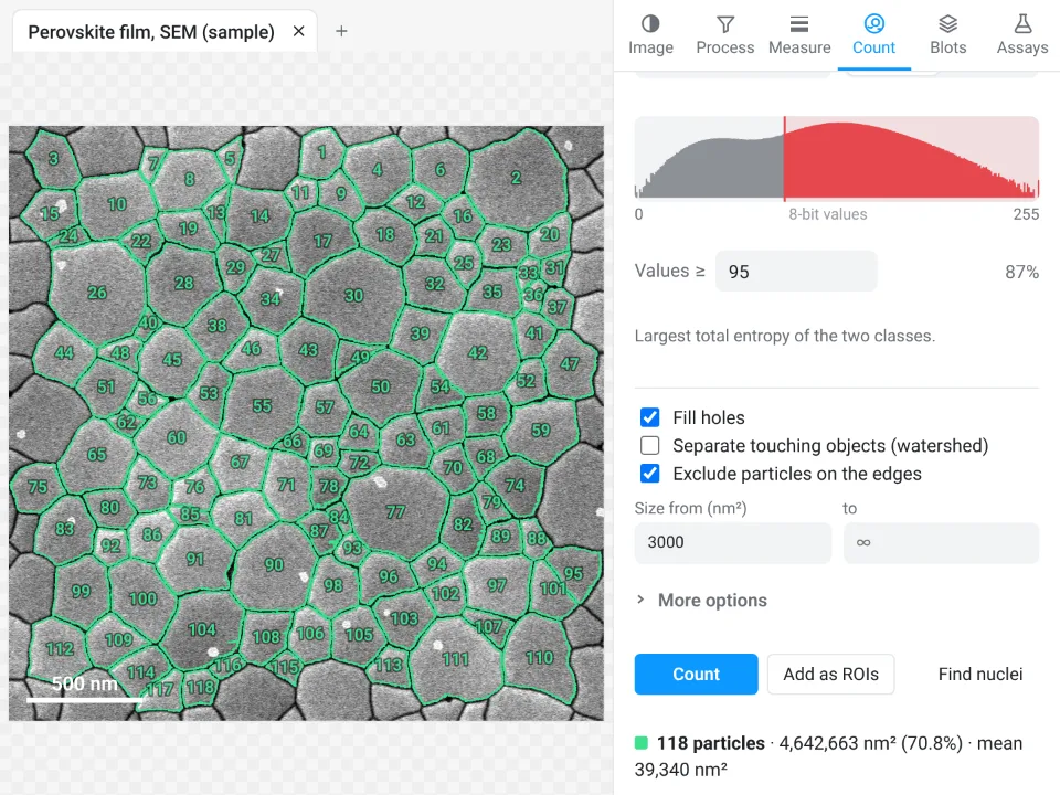
On the same film LabCanvas counts 118 grains with a mean area of 39,340 nm² (MaxEntropy cut at 95, as in ImageJ); ImageJ gave 118 grains and 39,344.6 nm². Both give an equivalent diameter of 224 nm and G = 21.6.
Why it is a good choice for grain size:
- Nothing to install: it runs in the browser on any computer or tablet.
- ImageJ's own names: the sixteen threshold methods, fill holes, exclude on edges, and a Summary row with Count, Total Area and Average Size.
- An image check flags JPEG compression, clipped pixels and uneven brightness before you count.
- Results go straight to Graphs for the histogram, and each table carries a methods sentence with the exact threshold value.
- Free with a LabCanvas account (CSV download is part of Pro); every measurement is checked in more than 4,000 automated tests.
It has no macro language (Count › Batch runs the same settings on many images) and does not read makers' own formats: export a TIFF first. Open Image Analysis.
ImageJ and Fiji are independent open-source projects; LabCanvas is not affiliated with them.
References
- ASTM International (2025). ASTM E112-25: Standard Test Methods for Determining Average Grain Size. doi:10.1520/E0112-25
- ASTM International (2023). ASTM E1382-97(2023): Standard Test Methods for Determining Average Grain Size Using Semiautomatic and Automatic Image Analysis. doi:10.1520/E1382-97R23
- Legland D, Arganda-Carreras I, Andrey P (2016). MorphoLibJ: integrated library and plugins for mathematical morphology with ImageJ. Bioinformatics 32(22): 3532–3534. doi:10.1093/bioinformatics/btw413
- Arganda-Carreras I, Kaynig V, Rueden C, et al. (2017). Trainable Weka Segmentation: a machine learning tool for microscopy pixel classification. Bioinformatics 33(15): 2424–2426. doi:10.1093/bioinformatics/btx180
Frequently asked questions
How do you calculate the ASTM grain size number from the mean grain area?
Convert the mean grain area
What is the formula for the intercept method?
Lay test lines of known total length
Can ImageJ measure grain size from an SEM image?
Yes. Set the scale from the scale bar, threshold the image so that every grain is a closed region, and run Analyze › Analyze Particles with Exclude on edges: you get the area, Feret diameter and shape of every whole grain, and the Summary gives the mean area. ImageJ does not report the ASTM grain size number itself; compute G from the mean area or the mean intercept with the E112 formulas.
Should I use watershed to separate grains?
Only where boundaries are open. Watershed splits merged round grains, but it also cuts elongated or irregular grains in two, which lowers the mean size. If the boundaries in your image are closed after thresholding, leave it off; if a few are open, close them by hand or use watershed and compare the counts before and after.
Why is my XRD (Scherrer) crystallite size smaller than the grain size from SEM?
They measure different things. The Scherrer size is the size of coherently diffracting domains, measured perpendicular to the diffracting planes (through the film thickness in a symmetric θ–2θ scan); one grain can hold several domains, peak broadening also comes from strain and the instrument, and the method loses sensitivity above about 100–200 nm. A top-view SEM grain size is the lateral size of each grain at the surface.
What grain size number does a nanocrystalline thin film have?
A very high one. A mean grain area of 1 µm² is G 17.0, and the 224 nm grains of the sample film here are G 21.6, well past the end of the E112 tables (G 14). For films, report the mean equivalent diameter with its spread and histogram, and give G as well only when a specification asks for it.
Try it in LabCanvas
Every app is free to start in your browser. Create an account and begin.
Start Image Analysis free in your browserKeep reading
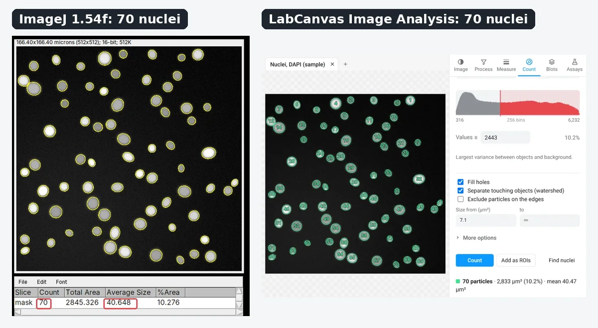
ImageJ vs LabCanvas Image Analysis: an honest comparison
ImageJ/Fiji or LabCanvas Image Analysis? Six everyday jobs done in both, six newer ones (macros, vendor files, 3D, StarDist, big images) and which to use.
How to use ImageJ: a beginner's tutorial for the 10 everyday jobs (2026)
How to use ImageJ and Fiji: get started, open an image, then 10 everyday jobs (scale, measure, threshold, count, background, blots) with exact menu paths.
How to set the scale and add a scale bar in ImageJ (with a calibration image to practise on)
Set the scale in ImageJ (Analyze › Set Scale) from a micrometer, scale bar or pixel size, add a scale bar, and practise on a free calibration image.