Deconvolution in ImageJ and Fiji: what it does and how to run it
What deconvolution does (the PSF, Richardson–Lucy), why FD Math Deconvolve fails on real images, and how to run Richardson–Lucy in ImageJ and Fiji.
Contents
Deconvolution sharpens a microscope image by undoing the blur of the optics, described by the point spread function (PSF). In plain ImageJ, Process › FFT › FD Math… with Operation: Deconvolve divides the image by the PSF in Fourier space, but on any image with noise it returns only noise. For real images use an iterative method such as Richardson–Lucy: in DeconvolutionLab2 (Plugins › DeconvolutionLab2, for ImageJ and Fiji), Iterative Deconvolve 3D, or the short ImageJ macro below, which runs Richardson–Lucy with FD Math.
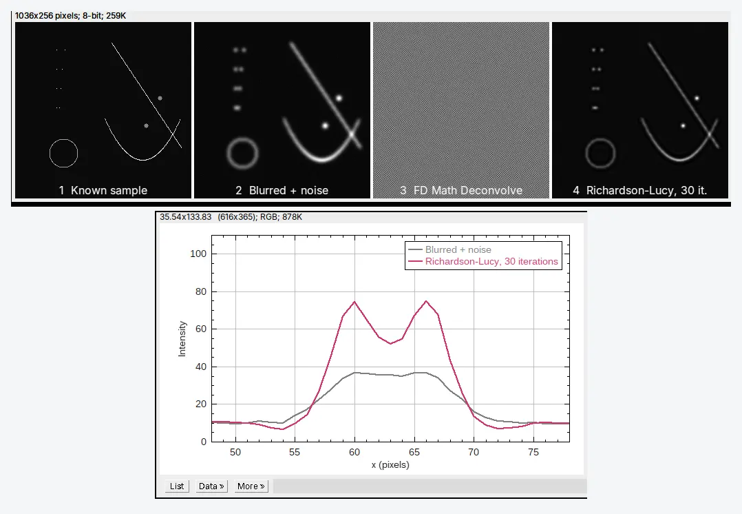
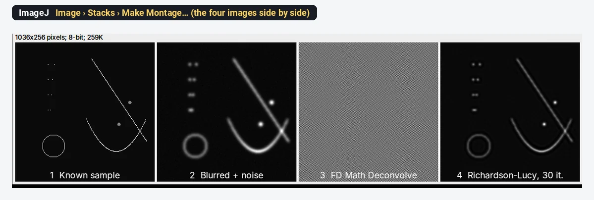
On a test image blurred with a known PSF, 30 Richardson–Lucy iterations separated two beads 6 pixels apart that the blurred image showed as one blob; the plain inverse filter turned the same image into noise of ±10⁹.
What you need: ImageJ 1.x or Fiji. Your image as 32-bit and a PSF image of the same size, centred and summing to 1 (for FD Math both must be square, 256 × 256, 512 × 512 and so on). The example is a synthetic test image made for this guide: beads, two filaments and a ring (256 × 256, 32-bit), blurred in ImageJ with a Gaussian PSF of 2.5 pixels sigma and with noise added. Time: 15 minutes.
Every picture is ImageJ 1.54f. DeconvolutionLab2 and Iterative Deconvolve 3D are plugins we did not run here; their steps are given in text.
What does deconvolution do?
A microscope never images a point as a point. It images it as a small blurred spot, the PSF; every point of the sample is spread out the same way, and the image is the sum of all those spots. Mathematically the image is the true sample convolved with the PSF, plus noise:
Deconvolution estimates the sample from the image and the PSF. Done well, it makes small objects smaller and brighter, separates objects that the blur merged, and in 3D pulls out-of-focus light back to where it came from. It cannot recover detail that the optics never passed, and it amplifies noise if pushed too far.
Do not confuse it with colour deconvolution (Image › Color › Colour Deconvolution in Fiji), which separates stains such as haematoxylin and DAB in brightfield images; see DAB IHC quantification.
Try the simple inverse in plain ImageJ (and see why it fails)
FD Math works on two images of the same square, power-of-2 size. To try it, you need an image and a PSF; here we make the blurred image ourselves from a known sample, so we know what the answer should be.
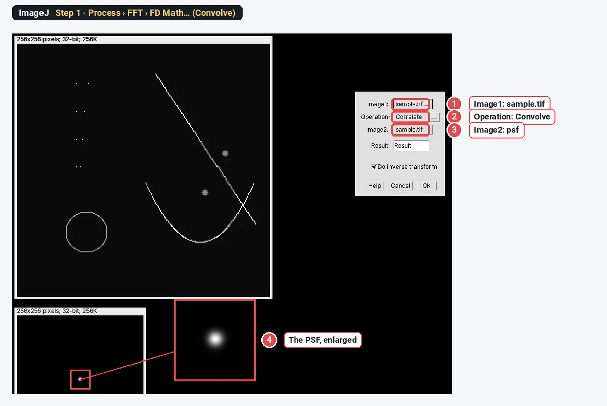
Step 1: Blur a known sample with the PSF
Open the sample and the PSF. Choose Process › FFT › FD Math…, set Image1 to the sample, Operation: Convolve, Image2 to the PSF, tick Do inverse transform, and name the result blurred. We then added noise with Process › Noise › Add Specified Noise… (SD 0.5) and set negatives to 0 with Process › Math › Min… (0), as a real camera image would have.
Step 2: Run FD Math Deconvolve
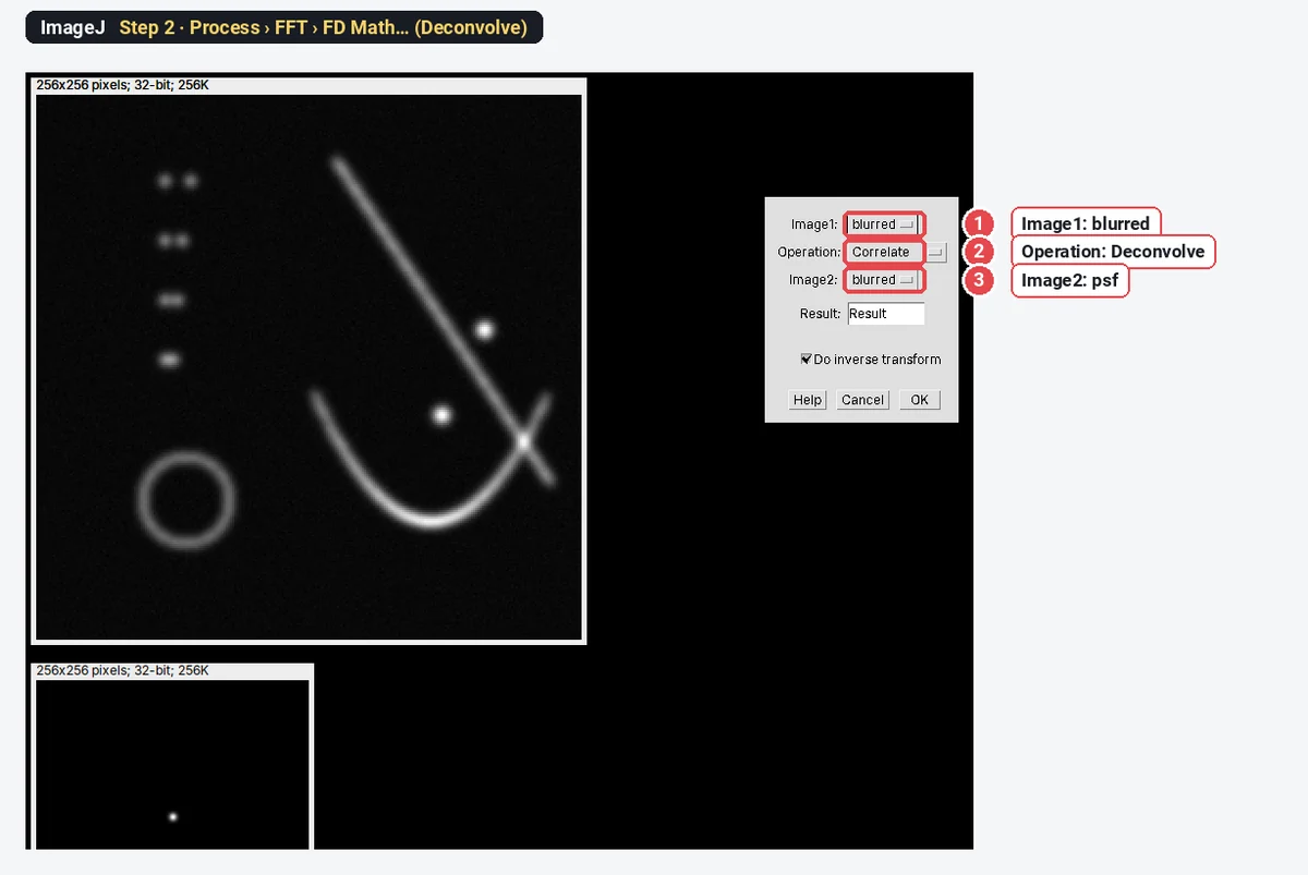
Open Process › FFT › FD Math… again: Image1 blurred, Operation: Deconvolve, Image2 the PSF, Do inverse transform ticked.
Step 3: Look at the result
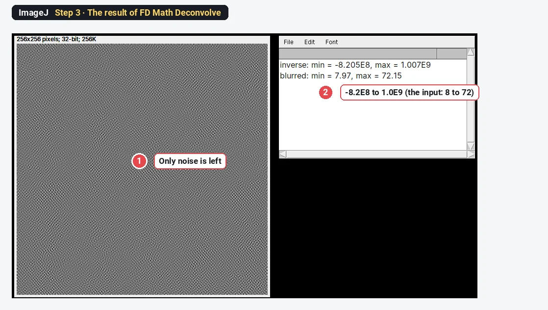
Deconvolve divides the image's Fourier transform by the PSF's. For a blurring PSF, that transform is almost zero at fine detail, and the noise sits exactly there: dividing by tiny numbers multiplies it by enormous ones. Even with no noise added, the plain inverse gave values from -3265 to 3479 for a sample that runs from 10 to 1010, from rounding errors alone. This is why nobody deconvolves real images with a plain inverse filter.
Richardson–Lucy in plain ImageJ, step by step
Richardson–Lucy (Richardson 1972; Lucy 1974) is the standard iterative method for fluorescence images. It starts from the blurred image as a guess and repeats one correction: blur the guess with the PSF, compare it with the measured image (divide), blur that ratio with the PSF, and multiply the guess by it. Each round sharpens a little, values never go negative, and the total intensity is kept. You can run it in plain ImageJ with FD Math and the Image Calculator.
Step 4: Run the Richardson–Lucy macro
Open the blurred image and rename it blurred; open the PSF and rename it psf (Image › Rename…). Both must be 32-bit and the same power-of-2 size, and the PSF must be centred, symmetric and sum to 1. Open Plugins › New › Macro, paste the macro, and click Run.
// Richardson-Lucy deconvolution with FD Math (plain ImageJ 1.x)
// Needs two open 32-bit images of the same power-of-2 size:
// "blurred" and "psf" (centred, symmetric, summing to 1).
n = 30;                                   // number of iterations
setBatchMode(true);
selectImage("blurred");
run("Duplicate...", "title=estimate");    // start from the blurred image
for (i = 1; i <= n; i++) {
  run("FD Math...", "image1=estimate operation=Convolve image2=psf result=reblurred do");
  run("Min...", "value=0.000001");        // avoid dividing by zero
  imageCalculator("Divide create 32-bit", "blurred", "reblurred");
  rename("ratio");
  run("FD Math...", "image1=ratio operation=Convolve image2=psf result=correction do");
  imageCalculator("Multiply 32-bit", "estimate", "correction");
  close("reblurred"); close("ratio"); close("correction");
}
selectImage("estimate");
rename("RL " + n + " iterations");
resetMinAndMax();
setBatchMode("exit and display");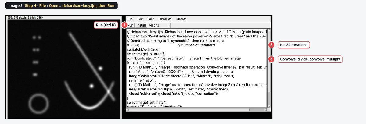
The macro uses the PSF for both blurring steps, which is correct only for a symmetric PSF (a Gaussian, or a centred Airy pattern). For an asymmetric PSF the second step needs the PSF rotated by 180°: use Image › Transform › Rotate 90 Degrees Right twice to make it.
Step 5: Check that it helped
Draw a Straight line across two close beads and compare the profiles (Analyze › Plot Profile, Ctrl K) of the blurred and the deconvolved image. Two objects count as resolved when the profile dips clearly between them.
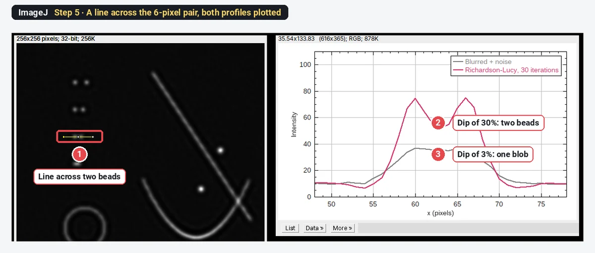
The result on the test image
| Bead pair (separation) | Dip between the beads, blurred | Dip after Richardson–Lucy, 30 iterations |
|---|---|---|
| 12 pixels | 61% | 94% |
| 8 pixels | 32% | 77% |
| 6 pixels | 3% (one blob) | 30% (two beads) |
| 4 pixels | none (one peak) | none (one peak) |
The PSF here is 5.9 pixels across at half height. Richardson–Lucy brought the limit down to about 6 pixels, but not to 4: deconvolution improves resolution modestly; it does not recover detail far below the PSF. The beads' peaks rose from 35–44 to 74–89, while the image mean stayed at 11.64. Look closely and you also see the side effect of iterating: a faint halo (ringing) around the ring and along the filaments.
Deconvolution with DeconvolutionLab2 (ImageJ and Fiji)
DeconvolutionLab2 (Sage et al. 2017) is the full-featured option: 2D and 3D, many algorithms, and a PSF you load or simulate. It is a plugin for ImageJ 1.x and Fiji; we describe it in text.
- Download DeconvolutionLab_2.jar from the EPFL Biomedical Imaging Group's DeconvolutionLab2 page. Do not unzip it; put it in the plugins folder of ImageJ or Fiji and restart.
- Open your image (a 2D image or a Z-stack, ideally 32-bit) and your PSF (a measured bead image, cropped and centred, or a theoretical PSF).
- Choose Plugins › DeconvolutionLab2 › DeconvolutionLab2 Lab for the full window: choose the image and the PSF, the algorithm (Richardson-Lucy to start, with its number of iterations), and the outputs, then run.
- For a macro, DeconvolutionLab2 Run takes a command line, with platform meaning an open image by its title:
run("DeconvolutionLab2 Run", " -image platform blurred -psf platform psf -algorithm RL 30");| Algorithm (short name) | When to use it |
|---|---|
| Richardson-Lucy (RL) | Fluorescence images, the usual first choice |
| Richardson-Lucy Total Variation (RLTV) | Noisy images: a regularisation term limits noise and ringing |
| Regularized Inverse Filter (RIF) | Fast, one step; a quick look |
| Tikhonov-Miller (TM), Landweber (LW), Non-negative least squares (NNLS, LW+) | Comparisons and special cases |
| Naive Inverse Filter (NIF) | The same as FD Math Deconvolve; only for noise-free tests |
Iterative Deconvolve 3D (Bob Dougherty's plugin, with its companion Diffraction PSF 3D to compute a theoretical PSF) is the other classic: a non-negative iterative method with an optional Wiener-filter step. For a 2D image use a single-plane PSF, and start with about 10 iterations.
Where do I get the PSF?
- Measured: image sub-resolution fluorescent beads (100–200 nm) with the same objective, immersion, wavelength and pixel size as your sample. Average several beads, subtract the background and crop around one, centred. This captures the real aberrations of your microscope.
- Theoretical: compute it from the numerical aperture, emission wavelength, refractive index, pixel size and (for 3D) slice spacing, with Diffraction PSF 3D or the PSF Generator plugin. It is easy but ignores aberrations.
- Never a guess. A PSF that is too wide over-sharpens and rings; one that is too narrow does little.
Pitfalls
- Saturated pixels. Clipped values are not the real intensity, so the blur cannot be undone there. Check the histogram first; see saturated pixels.
- Background left in. A constant offset (camera offset) breaks the model. Subtract it first.
- Too many iterations. Noise grows into speckle and halos appear. Compare a few iteration counts and choose one for the whole experiment.
- Wrong pixel size or spacing. The PSF must have the same pixel size (and Z spacing) as the image.
- Edges. FD Math treats the image as repeating at its edges, so objects near one edge can leak to the other. Pad the image if objects reach the edge.
- 8-bit images. Convert to 32-bit first (Image › Type › 32-bit).
- Comparing raw and deconvolved data. Measure every group the same way, all deconvolved with the same PSF and settings, or none.
Reporting it
Images were deconvolved in Fiji (ImageJ [1.54]) with DeconvolutionLab2 (Sage et al. 2017) using the Richardson–Lucy algorithm (Richardson 1972; Lucy 1974), [30] iterations, with a [measured PSF from 100 nm beads / theoretical PSF for NA 1.4, 520 nm]. All conditions were processed with identical settings. Intensities were measured on [raw / deconvolved] images.
Switch to LabCanvas: measure the deconvolved image
LabCanvas Image Analysis has no deconvolution (only colour deconvolution for stains). Deconvolve in ImageJ or Fiji, save the result as a TIFF (32-bit is fine), and measure it in the browser.
- Click Open an image and choose the TIFF; 32-bit values are measured as they are.
- Read the Image check: clipping, illumination and, for a stack, which slice is sharpest.
- Measure: a line and Profile in the Measure tab for resolution, ROIs and Measure for intensities, or Count › Count particles for objects.
- Send to Graphs to compare conditions.
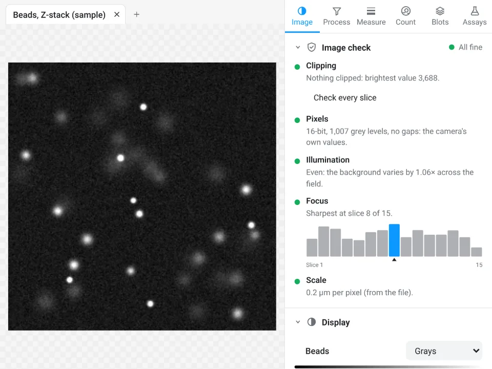
Why switch for the measuring:
- An image check before you measure: clipped pixels, JPEG compression and uneven light are flagged, the things that also spoil deconvolution.
- No install: ImageJ's measurements (Area, Mean, IntDen, Feret, Plot Profile) in the browser on any computer.
- Results straight to Graphs and a figure with a scale bar, with a methods sentence to copy.
ImageJ and Fiji stay the tools for the deconvolution itself.
Open Image Analysis: free with a LabCanvas account (downloading files is part of LabCanvas Pro). ImageJ and Fiji are independent open-source projects; LabCanvas is not affiliated with them.
References
- Lucy LB (1974). An iterative technique for the rectification of observed distributions. The Astronomical Journal 79, 745–754. doi:10.1086/111605
- Richardson WH (1972). Bayesian-based iterative method of image restoration. Journal of the Optical Society of America 62, 55–59. doi:10.1364/JOSA.62.000055
- Sage D, Donati L, Soulez F, Fortun D, Schmit G, Seitz A, Guiet R, Vonesch C, Unser M (2017). DeconvolutionLab2: an open-source software for deconvolution microscopy. Methods 115, 28–41. doi:10.1016/j.ymeth.2016.12.015
- Schindelin J, Arganda-Carreras I, Frise E, et al. (2012). Fiji: an open-source platform for biological-image analysis. Nature Methods 9, 676–682. doi:10.1038/nmeth.2019
- Schneider CA, Rasband WS, Eliceiri KW (2012). NIH Image to ImageJ: 25 years of image analysis. Nature Methods 9, 671–675. doi:10.1038/nmeth.2089
Frequently asked questions
How do I deconvolve an image in ImageJ?
Plain ImageJ 1.x has Process › FFT › FD Math with the operation Deconvolve, which divides the image by the PSF in Fourier space. It only works on noise-free test images. For real images use an iterative method: Richardson–Lucy with DeconvolutionLab2 (Plugins › DeconvolutionLab2) or Iterative Deconvolve 3D, both plugins for ImageJ and Fiji, or the short Richardson–Lucy macro in this guide.
What is a point spread function (PSF)?
The PSF is the image of a single point of light through your microscope: a small blurred spot in 2D, an hourglass shape in 3D. Every image is the true sample convolved with the PSF. You get it by imaging sub-resolution fluorescent beads with the same objective and settings, or by computing a theoretical PSF from the wavelength, numerical aperture, refractive index and pixel size.
Why does FD Math Deconvolve give only noise?
It divides by the Fourier transform of the PSF, which is almost zero at high spatial frequencies. Noise lives exactly there, so dividing by numbers close to zero multiplies the noise by enormous factors. On the test image here, a blurred image with values from 8 to 72 came back with values from -8.2 × 10⁸ to 1.0 × 10⁹.
How many Richardson–Lucy iterations should I use?
Enough to sharpen, not so many that noise and ringing grow: often 10 to 50 for widefield images. Run a few counts (for example 10, 30, 100) on one image and compare; stop when structures you know are real stop improving. On the test image here, 30 iterations resolved two beads 6 pixels apart (a 30% dip between them, against 3% before).
Can I measure intensities after deconvolution?
Richardson–Lucy keeps the total intensity (on the test image the mean stayed at 11.64), so integrated intensities of whole objects can be compared if every image is deconvolved with the same PSF and iterations. Peak values and local contrast change, and ringing can create dark halos, so state that measurements were made on deconvolved images, or measure intensities on the raw data and use the deconvolved image for shapes and positions.
Does Fiji have deconvolution built in?
Not as a menu command for everyday use. Install DeconvolutionLab2 (a jar from the EPFL Biomedical Imaging Group, placed in the plugins folder) or Iterative Deconvolve 3D; both run in ImageJ 1.x and Fiji. For GPU deconvolution of large 3D data, dedicated tools outside ImageJ are faster.
Try it in LabCanvas
Every app is free to start in your browser. Create an account and begin.
Start Image Analysis free in your browserKeep reading
ImageJ vs LabCanvas Image Analysis: an honest comparison
ImageJ/Fiji or LabCanvas Image Analysis? Six everyday jobs done in both, six newer ones (macros, vendor files, 3D, StarDist, big images) and which to use.
How to use ImageJ: a beginner's tutorial for the 10 everyday jobs (2026)
How to use ImageJ and Fiji: get started, open an image, then 10 everyday jobs (scale, measure, threshold, count, background, blots) with exact menu paths.
How to set the scale and add a scale bar in ImageJ (with a calibration image to practise on)
Set the scale in ImageJ (Analyze › Set Scale) from a micrometer, scale bar or pixel size, add a scale bar, and practise on a free calibration image.