Wound healing (scratch) assay analysis in ImageJ: % closure step by step
Measure a scratch wound in ImageJ: variance filter, threshold and Analyze Particles per frame, then % closure and closure rate, with a worked example.
Contents
To analyse a scratch (wound healing) assay in ImageJ, measure the open, cell-free area of the gap in every frame: convert the time-lapse to 32-bit, run Process › Filters › Variance… (radius about one cell) so the textured cells turn bright and the smooth gap stays dark, threshold the gap with Image › Adjust › Threshold…, and run Analyze › Analyze Particles… with Summarize on all frames. Then:
and the closure rate is the slope of open area against time (µm² per hour).
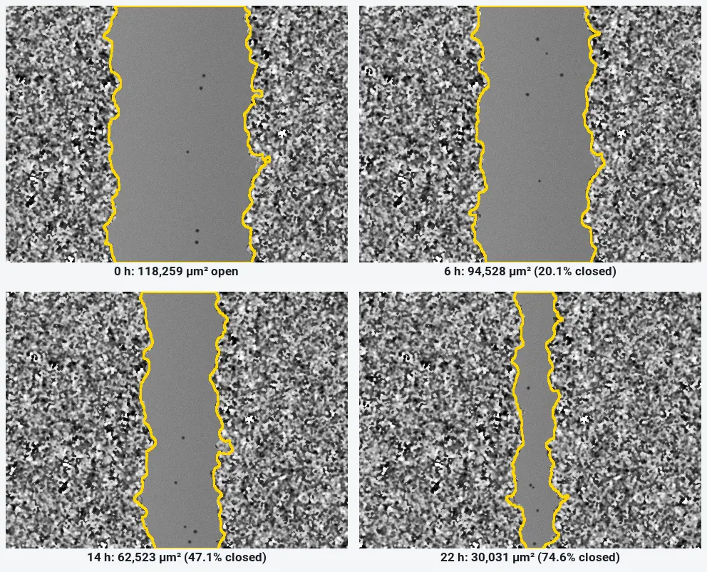
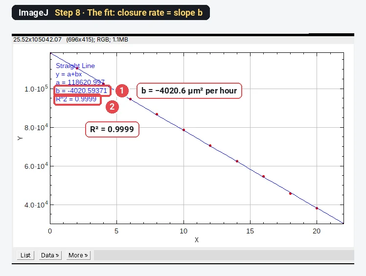
On the worked example below, ImageJ measures the gap closing from 118,259 µm² to 30,031 µm² in 22 hours: 74.6% closure at 4,021 µm² per hour (R² 0.9999).
What you need: ImageJ 1.x or Fiji (every command here is in both). A time-lapse of one field of a scratch, or one image per time point of the same field; set the pixel size if the file has none. The example is a synthetic scratch time-lapse (12 frames 2 h apart, 480 × 360 pixels, 1.3 µm per pixel) made for practice, with a known open area in every frame. Time: about 15 minutes.
Why a variance filter finds the gap
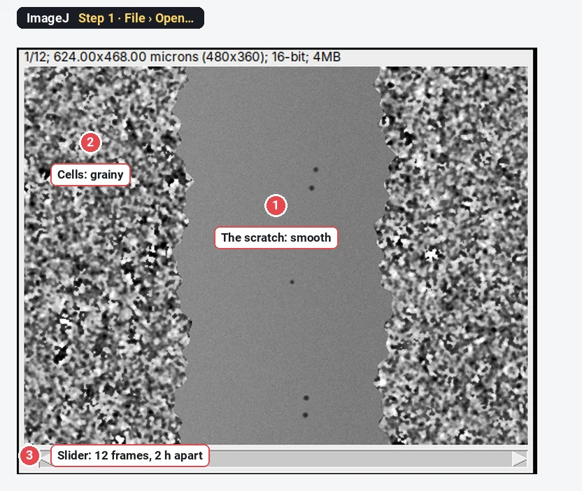
A phase-contrast or brightfield image of cells is grainy: cell edges, nuclei and organelles make the grey value jump from pixel to pixel. The scratch has no cells, so it is smooth. The mean brightness of the two can be almost the same, which is why a plain threshold of the image fails.
The variance filter replaces each pixel by the variance of the grey values in a small circle around it. Grainy regions get a high value, smooth regions a low one. A threshold of the variance image then separates cells from gap. This is the idea behind the MRI Wound Healing Tool and the Wound Healing Size Tool (Suarez-Arnedo et al. 2020).
How do I measure the wound area in ImageJ? Step by step
Step 1: Open the time-lapse
Click File › Open… and choose the file. Check the line above the image: it should show the size in microns (here 624.00x468.00 microns), and the slider at the bottom should run through all frames. If the frames came as separate files, use File › Import › Image Sequence… to make one stack. If the scale is missing, set it with Analyze › Set Scale….
Step 2: Run the variance filter
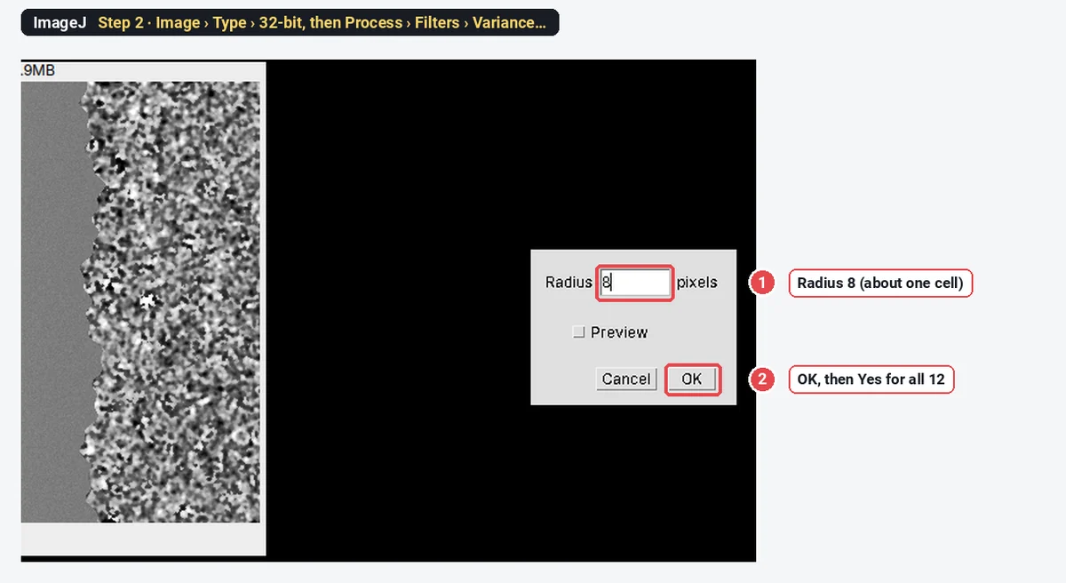
Make a copy for the analysis (Image › Duplicate…, tick Duplicate stack), then choose Image › Type › 32-bit so the variance does not clip at the top of the 16-bit range. Now choose Process › Filters › Variance…, type a Radius of about one cell (8 pixels here, about 10 µm), click OK, and answer Yes to process all 12 images.
Step 3: Look at the variance image
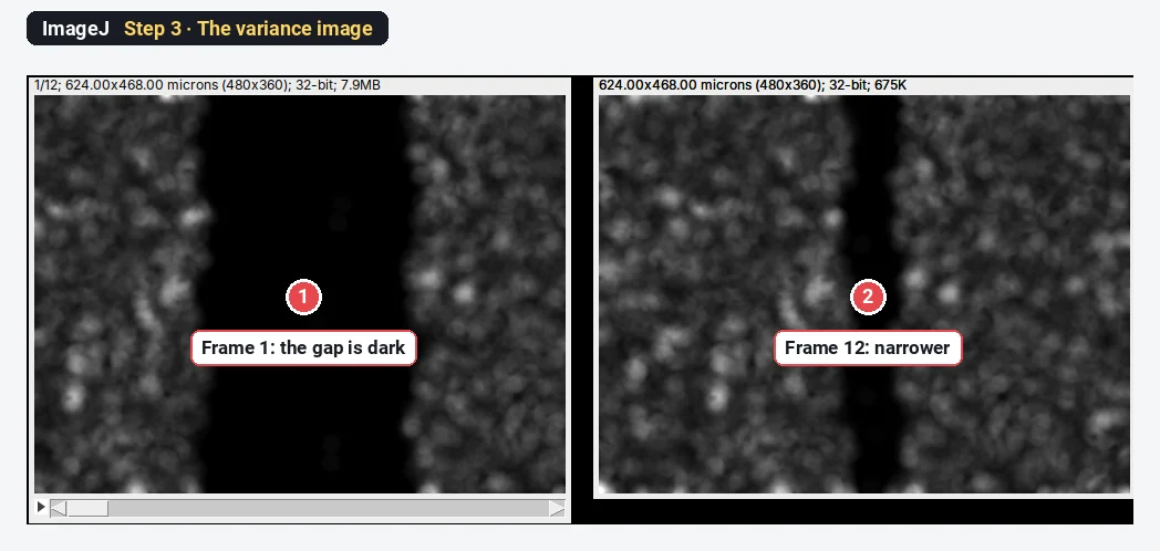
The cells are now bright and the gap black. Step through the frames: the black band narrows as the two fronts move in.
Step 4: Threshold the gap
Go back to frame 1 (the widest gap) and choose Image › Adjust › Threshold…. Pick Otsu, and untick Dark background: the gap is the dark part you want selected. The gap turns red, with a few small red specks between cells. Do not click Apply; leave the window open so the threshold stays set for every frame.
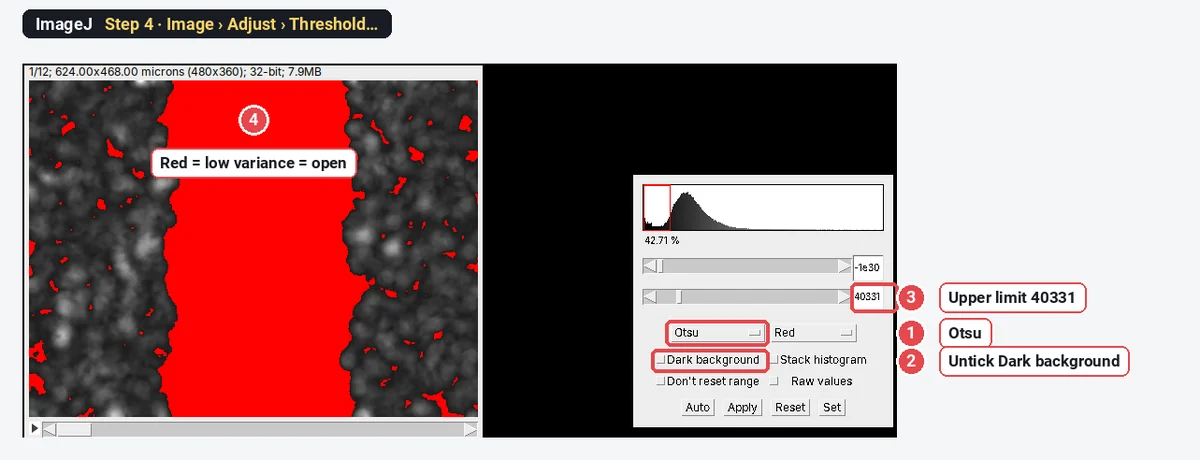
Keep the same threshold for all frames. If you let ImageJ pick a new one per frame, a narrower gap gets a different cut, and the areas are no longer comparable.
Step 5: Analyze Particles on all frames
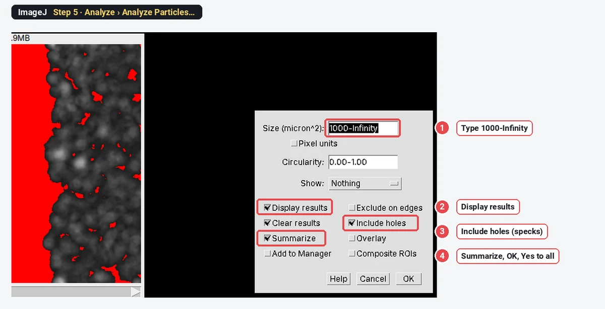
Choose Analyze › Analyze Particles…. Type a minimum Size that is larger than the specks and smaller than the gap (1000-Infinity µm² here), tick Display results, Include holes (debris inside the gap counts as open) and Summarize, and click OK. Answer Yes to process all 12 images.
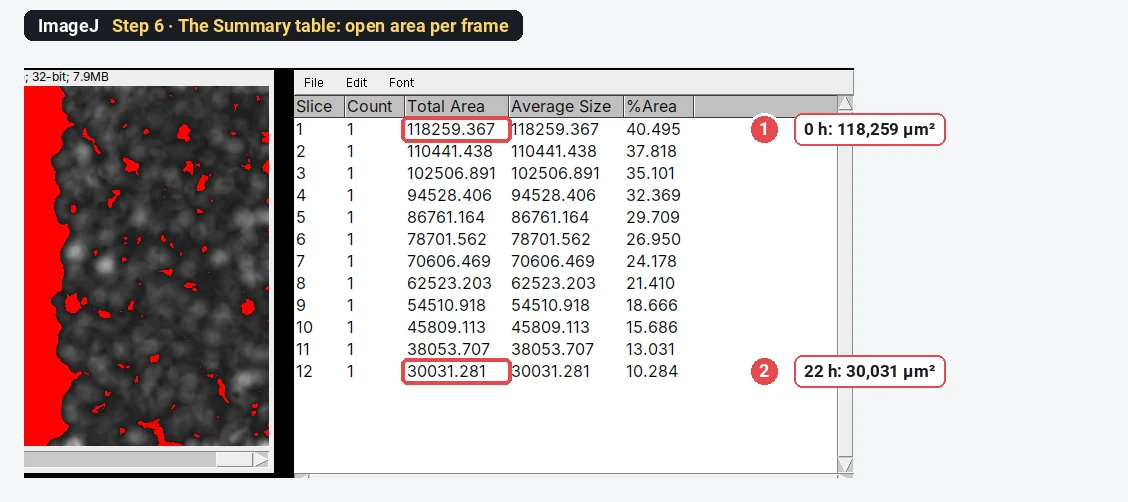
Step 6: Read the open area per frame
The Summary table has one row per frame. Total Area is the open area in µm²; %Area is the share of the field. Copy the table into a spreadsheet, or keep going in ImageJ.
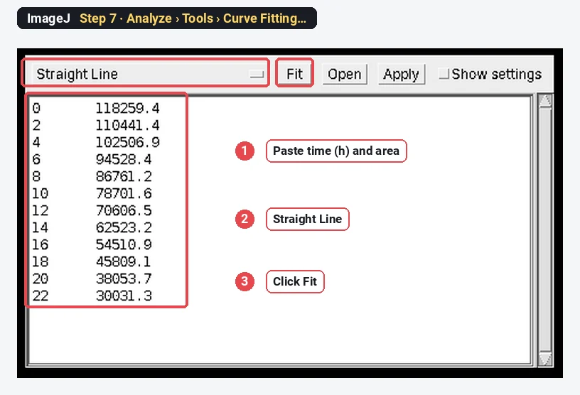
Step 7: Fit the closure rate
Choose Analyze › Tools › Curve Fitting…. Delete the example numbers, paste two columns (time in hours, open area), choose Straight Line and click Fit.
Step 8: Read the slope
The plot shows the points and the line, with the fitted a (intercept) and b (slope). The slope is the closure rate: here
The worked example: % closure and closure rate
Open area from the Summary table, with
| Frame | Time (h) | Open area (µm²) | % of initial | % closure | Mean width (µm) |
|---|---|---|---|---|---|
| 1 | 0 | 118,259 | 100.0 | 0.0 | 252.7 |
| 2 | 2 | 110,441 | 93.4 | 6.6 | 236.0 |
| 3 | 4 | 102,507 | 86.7 | 13.3 | 219.0 |
| 4 | 6 | 94,528 | 79.9 | 20.1 | 202.0 |
| 5 | 8 | 86,761 | 73.4 | 26.6 | 185.4 |
| 6 | 10 | 78,702 | 66.5 | 33.5 | 168.2 |
| 7 | 12 | 70,606 | 59.7 | 40.3 | 150.9 |
| 8 | 14 | 62,523 | 52.9 | 47.1 | 133.6 |
| 9 | 16 | 54,511 | 46.1 | 53.9 | 116.5 |
| 10 | 18 | 45,809 | 38.7 | 61.3 | 97.9 |
| 11 | 20 | 38,054 | 32.2 | 67.8 | 81.3 |
| 12 | 22 | 30,031 | 25.4 | 74.6 | 64.2 |
% closure at 22 h
Closure rate (slope of area against time) = 4,021 µm²/h, R² 0.9999. Divided by the wound length (468 µm), the gap narrows by 8.59 µm/h, so each front moves at about 4.3 µm/h.
Because the sample is synthetic, the true answer is known: the gap closes from 116,728 to 29,132 µm², 75.0% closure at 3,982 µm²/h. ImageJ's 74.6% and 4,021 µm²/h are within 1% of it. The variance window reaches across the cell front, so the outline sits a few pixels off the true edge; it is the same offset in every frame, which is why % closure and the rate come out right.
Or outline the gap by hand (polygon tool)
For a few images, or when the texture method fails (dense debris, very flat cells), outline the gap yourself. Pick the Polygon selections tool, click along one edge from top to bottom and back up the other edge, double-click to close, and press Ctrl M (Analyze › Measure). Set Area in Analyze › Set Measurements… first.
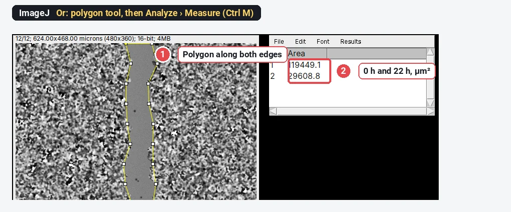
The polygon gives 75.2% closure here. It is quick for a handful of images, but it depends on the person clicking; if you do it by hand, blind yourself to the condition and outline every frame the same way.
The Wound Healing Size Tool plugin
The Wound Healing Size Tool (Suarez-Arnedo et al. 2020) packages the same variance-and-threshold idea for ImageJ and Fiji. Download it from its GitHub page, install it with Plugins › Macros › Install…, set the scale, and run it on an image or a stack. It reports the wound area, the area fraction, the mean wound width and the width's standard deviation, and it corrects the width for a tilted scratch. Its main settings are the variance window radius and the threshold value; check the outline on every image before you trust the numbers. The older MRI Wound Healing Tool macro works in a similar way.
Pitfalls
- Different fields at different times. Closure only means something for the same field. Mark the plate, use the stage memory, or align the frames before measuring.
- A new threshold for every frame. Keep the threshold from the first frame. An automatic threshold on each frame changes with the gap width.
- Window radius. Too small and the gap gets grainy holes from noise; too large and the outline moves away from the front. About one cell diameter works.
- Cells in the gap. Single cells that wander into the gap make holes in the open area. Include holes counts them as open, which is usually what the assay means (the front has not arrived).
- Proliferation. Over 24 h cells also divide, so closure is migration plus growth. Use mitomycin C or low serum if you want migration alone, and say which.
- % closure from different starting widths. A 400 µm scratch and a 600 µm scratch at the same speed give different % closure. Report the rate as well, or start from matched widths.
Reporting it
Scratch wounds were imaged every [2] h for [22] h ([10×], [1.3] µm per pixel). The open area was measured in ImageJ 1.54f: 32-bit, variance filter (radius [8] pixels), Otsu threshold of the first frame applied to all frames, Analyze Particles (minimum [1000] µm², holes included). % closure = (A₀ − Aₜ)/A₀ × 100; the closure rate is the slope of a linear fit of open area against time. Values are mean ± SD of [n] wells from [3] independent experiments.
Cite ImageJ (Schneider et al. 2012), and the Wound Healing Size Tool (Suarez-Arnedo et al. 2020) if you used it. Jonkman et al. (2014) give good general guidance on running and imaging the assay. Plot % closure against time per condition, with the rate per well as points.
Switch to LabCanvas: wound closure in a few clicks
LabCanvas Image Analysis has a guided wound healing assay in the browser: no plugin, no macro, nothing to install.
- Open the time-lapse (or click Try it on a sample for the same synthetic scratch) and go to Assays › Wound healing (scratch).
- Texture: a Window radius about one cell and a Threshold method; keep Same threshold for every frame and Correct the edges for the window ticked.
- Open area: Keep the region Reaching the edge, a smallest size, and Fill specks inside the wound.
- Click Measure all frames: open area, % of initial, % closure and mean width per frame, and the closure rates with R². Send the table to Graphs.
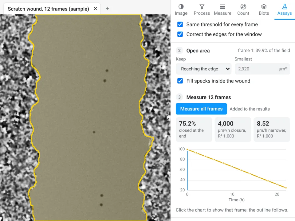
On the same synthetic scratch LabCanvas gives 75.2% closed by the last frame, closing at 4,000 µm²/h (R² 1.000), and 8.52 µm/h narrower; ImageJ above gave 74.6%, 4,021 µm²/h and 8.59 µm/h, against a true 75.0% and 3,982 µm²/h.
Why switch for scratch assays:
- A guided assay instead of a plugin: the variance method, one threshold for all frames and the edge correction are built in, with the outline drawn on every frame.
- Rates with R² straight away, and the table goes to Graphs for statistics across wells and a figure.
- Nothing to install: runs in the browser on any computer, next to the incubator microscope.
Fiji stays better for batch runs over hundreds of plates with a macro, and for files that need Bio-Formats (.czi, .nd2, .lif), which LabCanvas needs as OME-TIFF first.
Open Image Analysis: free with a LabCanvas account (downloading files is part of LabCanvas Pro). ImageJ and Fiji are independent open-source projects; LabCanvas is not affiliated with them.
References
- Jonkman JEN, Cathcart JA, Xu F, Bartolini ME, Amon JE, Stevens KM, Colarusso P (2014). An introduction to the wound healing assay using live-cell microscopy. Cell Adhesion & Migration 8, 440–451. doi:10.4161/cam.36224
- Schneider CA, Rasband WS, Eliceiri KW (2012). NIH Image to ImageJ: 25 years of image analysis. Nature Methods 9, 671–675. doi:10.1038/nmeth.2089
- Suarez-Arnedo A, Torres Figueroa F, Clavijo C, Arbeláez P, Cruz JC, Muñoz-Camargo C (2020). An ImageJ plugin for the high throughput image analysis of in vitro scratch wound healing assays. PLOS ONE 15, e0232565. doi:10.1371/journal.pone.0232565
Frequently asked questions
How do I calculate % wound closure?
How do I measure a scratch assay in ImageJ?
Convert the time-lapse to 32-bit, run Process › Filters › Variance… (radius about one cell) on all frames, threshold the low-variance gap with Image › Adjust › Threshold (Otsu, Dark background unticked), and run Analyze › Analyze Particles with a minimum size, Include holes and Summarize. The Summary table gives the open area of every frame. For a few images, outlining the gap with the polygon tool and pressing Ctrl M works too.
What is the Wound Healing Size Tool?
An ImageJ/Fiji plugin by Suarez-Arnedo et al. (PLOS ONE, 2020) that measures the wound area, the area fraction, the mean wound width and its standard deviation, from single images or stacks. It is installed with Plugins › Macros › Install… and uses the same idea as this guide: a variance filter separates the textured cells from the smooth gap.
How do I calculate the wound closure rate?
Plot the open area against time and fit a straight line (Analyze › Tools › Curve Fitting…, Straight Line). The slope is the closure rate in µm² per hour. Divide it by the length of the wound in the field to get the rate at which the gap narrows (µm per hour), and by 2 for the speed of each front.
Should I report % closure or the rate?
Both, if you can. % closure at a fixed time is easy to compare but depends on the starting width; the rate from a fit over several time points uses all the data and does not depend on one frame. Always say how the area was measured and at which times.
Is there a way to do this without installing ImageJ?
LabCanvas Image Analysis has a guided Wound healing (scratch) assay in the browser: it finds the gap from the texture on every frame and gives % closure and the closure rate with R². It is free with a LabCanvas account.
Try it in LabCanvas
Every app is free to start in your browser. Create an account and begin.
Start Image Analysis free in your browserKeep reading
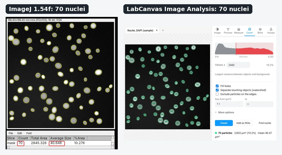
ImageJ vs LabCanvas Image Analysis: an honest comparison
ImageJ/Fiji or LabCanvas Image Analysis? Six everyday jobs done in both, six newer ones (macros, vendor files, 3D, StarDist, big images) and which to use.
How to use ImageJ: a beginner's tutorial for the 10 everyday jobs (2026)
How to use ImageJ and Fiji: get started, open an image, then 10 everyday jobs (scale, measure, threshold, count, background, blots) with exact menu paths.
How to set the scale and add a scale bar in ImageJ (with a calibration image to practise on)
Set the scale in ImageJ (Analyze › Set Scale) from a micrometer, scale bar or pixel size, add a scale bar, and practise on a free calibration image.