FRAP analysis in ImageJ: mobile fraction and half-time, step by step
FRAP in ImageJ: bleach, reference and background ROIs, Multi Measure, double normalisation, an exponential recovery fit, then the mobile fraction and t½.
Contents
To analyse FRAP in ImageJ, draw three ROIs (the bleached spot, the whole cell as reference and a background area), add them to the ROI Manager, and use More › Multi Measure to get their mean intensity in every frame. Double normalise the bleach-spot curve, fit the recovery with Analyze › Tools › Curve Fitting… (Exponential Recovery,
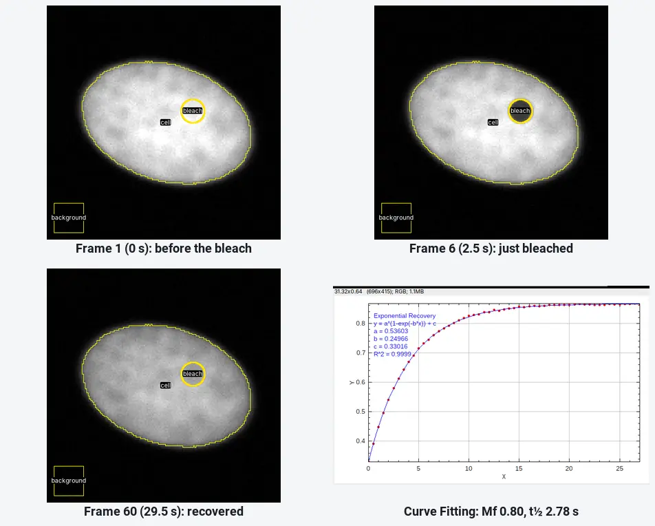
On the worked example below ImageJ gives
What you need: ImageJ 1.x or Fiji (every command here is in both). A FRAP time-lapse as one stack with a few frames before the bleach, and the frame interval. The example is a synthetic FRAP movie (60 frames at 0.5 s, 160 × 160 pixels, 0.1 µm per pixel, bleached after frame 5) made for practice, with a known mobile fraction (0.8) and recovery rate (0.25 s⁻¹). Time: about 20 minutes.
What the mobile fraction and t½ mean
In FRAP (fluorescence recovery after photobleaching) you bleach the fluorescent protein in a small spot and watch fresh, unbleached protein move back in.
- The half-time (t½) is how long the spot takes to recover half of what it will recover. Shorter means faster exchange or diffusion.
- The mobile fraction (Mf) is the share of the bleached protein that is replaced. If the spot comes back to 80% of the way between the post-bleach level and the pre-bleach level,
How do I measure FRAP in ImageJ? Step by step
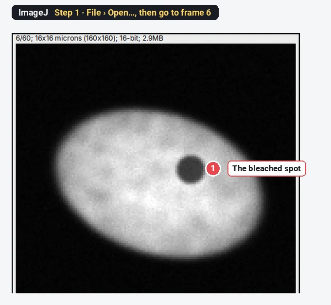
Step 1: Open the movie and find the bleach
Click File › Open… and choose the movie. Step through it with the slider and note the last frame before the bleach (frame 5 here) and the first frame after it (frame 6, where the spot is dark). Check the frame interval under Image › Properties… (0.5 s here).
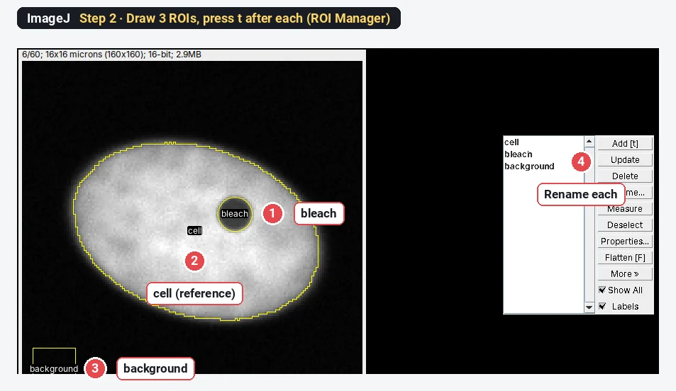
Step 2: Draw the three ROIs and add them to the ROI Manager
Open Analyze › Tools › ROI Manager…. Then draw each region and press t to add it:
- bleach: the Oval tool, a circle exactly on the bleached spot (draw it on the first post-bleach frame, where you can see it).
- cell: the whole cell, as reference. Trace it with the Freehand tool, or threshold frame 1 (Image › Adjust › Threshold…, Otsu, Dark background) and Edit › Selection › Create Selection.
- background: a square outside the cell, away from other cells.
Select each entry and click Rename… to call them bleach, cell and background; the names become the column titles.
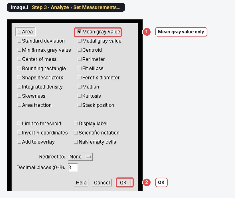
Step 3: Measure the mean only
Choose Analyze › Set Measurements… and tick Mean gray value only (untick Area and the rest), so the table stays readable. Click OK.
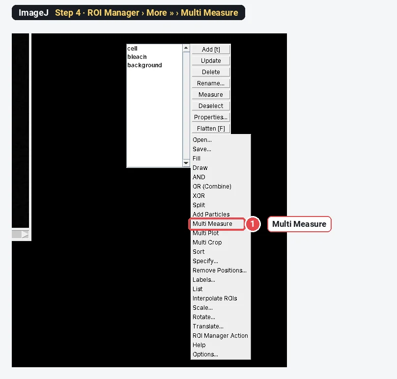
Step 4: Multi Measure
Click in the ROI Manager's list without selecting anything (or click Deselect), then More » and Multi Measure.
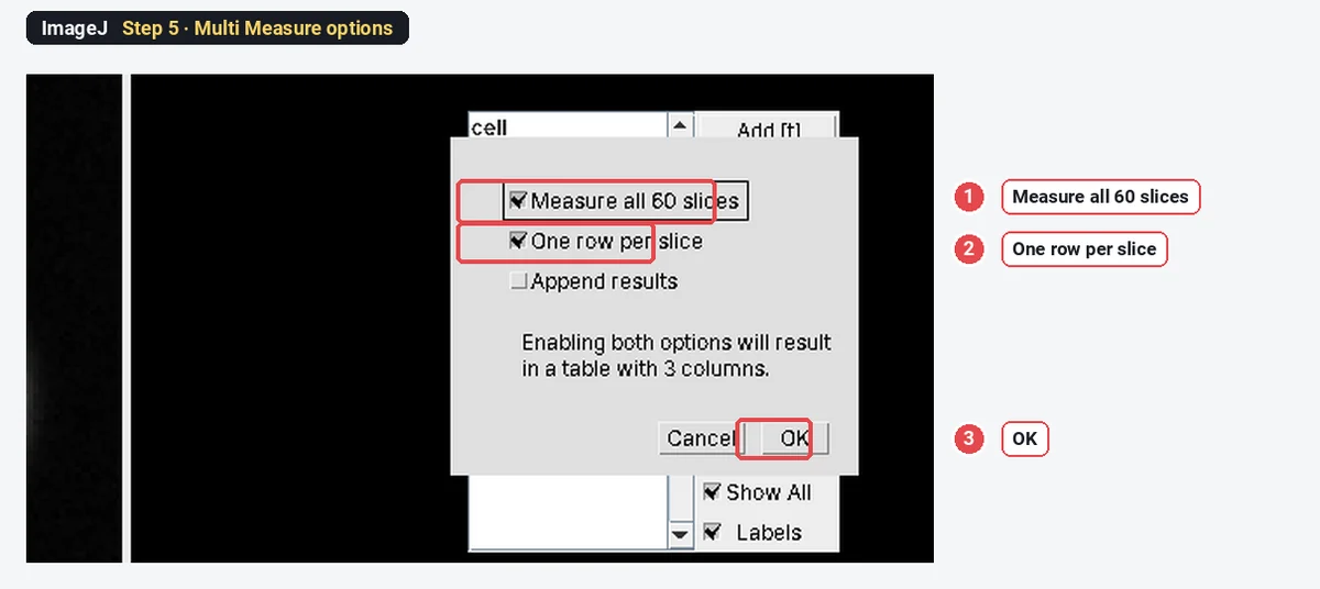
Step 5: Set the Multi Measure options
Tick Measure all 60 slices and One row per slice, leave Append results unticked, and click OK.
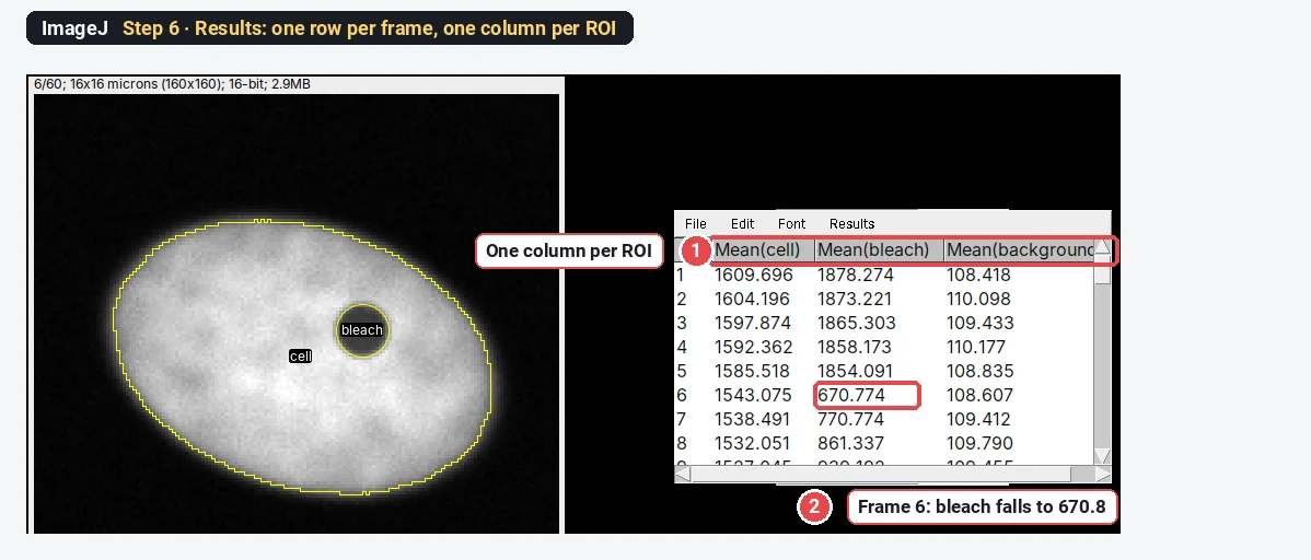
Step 6: Read the raw intensities
The Results table has one row per frame and one column per ROI: Mean(cell), Mean(bleach) and Mean(background). At frame 6 the bleach column drops from about 1854 to 671.
Step 7: Double normalise
Open Plugins › New › Macro, paste the macro below, set nPre (frames before the bleach) and dt (seconds per frame), and click Run. It adds a Time (s) and a Norm column to the Results table and plots the normalised curve.
// FRAP double normalisation (run on the Results table from Multi Measure)
nPre = 5;      // frames before the bleach
dt = 0.5;      // seconds per frame
n = nResults;
F = Table.getColumn("Mean(bleach)");
R = Table.getColumn("Mean(cell)");
B = Table.getColumn("Mean(background)");
Fpre = 0; Rpre = 0;
for (i = 0; i < nPre; i++) { Fpre += F[i] - B[i]; Rpre += R[i] - B[i]; }
Fpre /= nPre; Rpre /= nPre;
for (i = 0; i < n; i++) {
  setResult("Time (s)", i, i * dt);
  setResult("Norm", i, (Rpre / (R[i] - B[i])) * ((F[i] - B[i]) / Fpre));
}
updateResults();
Plot.create("FRAP", "Time (s)", "Normalised intensity");
Plot.add("circle", Table.getColumn("Time (s)"), Table.getColumn("Norm"));
Plot.setLimits(0, n * dt, 0, 1.1);
Plot.show();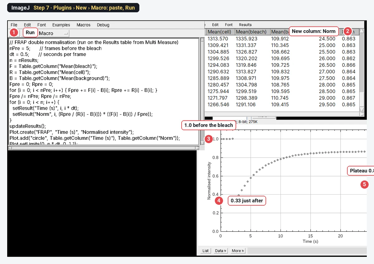
The formula, for each frame
The second factor scales the spot to its own pre-bleach level. The first corrects for fluorescence lost from the whole cell, both in the bleach and through imaging. This is the double normalisation of Phair, Gorski and Misteli (2004).
Step 8: Fit the recovery
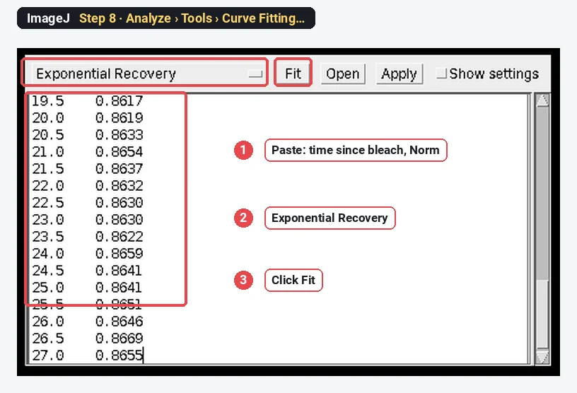
Copy the Time (s) and Norm columns from the first post-bleach frame (frame 6) to the end, and subtract the time of frame 6 so the recovery starts at 0 s. Choose Analyze › Tools › Curve Fitting…, delete the example numbers, paste the two columns, choose Exponential Recovery from the list, and click Fit.
Step 9: Read a, b and c
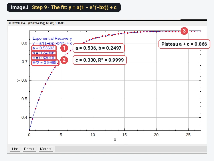
ImageJ plots the fit and lists the parameters of
The worked example: Mf and t½ by hand
Part of the Results table (background-subtracted pre-bleach means:
| Frame | Time (s) | Mean(bleach) | Mean(cell) | Mean(background) | Norm |
|---|---|---|---|---|---|
| 1 | 0.0 | 1878.3 | 1609.7 | 108.4 | 0.999 |
| 5 | 2.0 | 1854.1 | 1585.5 | 108.8 | 1.002 |
| 6 | 2.5 | 670.8 | 1543.1 | 108.6 | 0.332 |
| 7 | 3.0 | 770.8 | 1538.5 | 109.4 | 0.392 |
| 8 | 3.5 | 861.3 | 1532.1 | 109.8 | 0.448 |
| 11 | 5.0 | 1071.6 | 1516.4 | 109.9 | 0.580 |
| 16 | 7.5 | 1272.3 | 1488.1 | 110.9 | 0.715 |
| 21 | 10.0 | 1357.4 | 1461.2 | 110.3 | 0.782 |
| 31 | 15.0 | 1405.1 | 1408.5 | 109.9 | 0.845 |
| 60 | 29.5 | 1291.1 | 1266.5 | 109.4 | 0.865 |
Frame 6, worked through:
From the fit (Step 9):
- Mobile fraction
- t½
The sample was made with
Why the reference ROI matters: single vs double normalisation
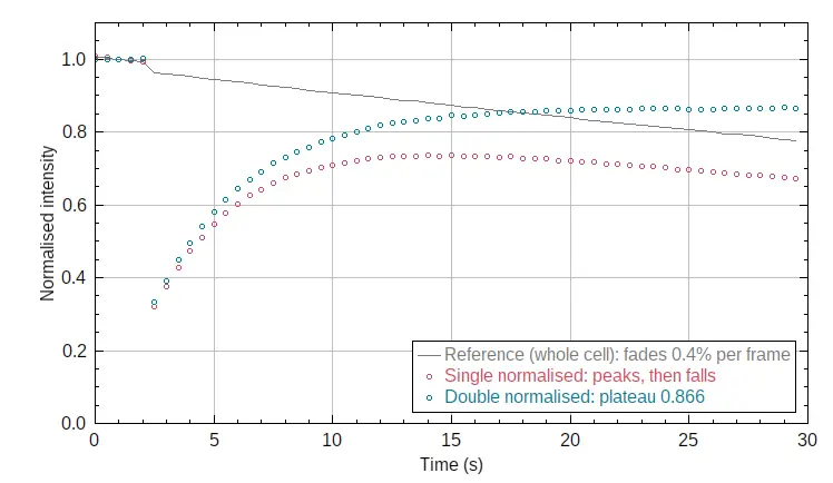
The raw bleach-spot intensity, divided only by its own pre-bleach level (single normalisation), mixes recovery with bleaching from imaging. Here the whole cell fades 0.4% per frame, so the single-normalised curve rises, peaks near 15 s and then falls:
| Normalisation | Mf | t½ (s) |
|---|---|---|
| Single (spot only) | 0.60 | 1.73 |
| Double (spot and whole-cell reference) | 0.80 | 2.78 |
| True value of the sample | 0.80 | 2.77 |
Without the reference, both numbers are wrong: the fit catches the early rise and treats the fading as a lower plateau.
Pitfalls
- Too few pre-bleach frames. Take at least 3 to 5; Fpre is their mean.
- A bleach ROI bigger or smaller than the bleached spot. Draw it on the first post-bleach frame, the size of the dark spot.
- The cell moves. Check the ROIs on the last frame. Register the stack first if the cell drifts.
- Reference not the whole cell. The reference must contain the whole pool that exchanges with the spot (the whole nucleus for a nuclear protein).
- Fitting the pre-bleach frames. Fit from the first post-bleach frame, with time starting at 0 there.
- A bad single exponential fit. If the residuals curve, the protein may have two populations; try a double exponential (a custom fit in Curve Fitting) and say so.
- t½ is not a diffusion coefficient. Converting t½ to D needs a model for the spot size and bleach profile (for a circular spot, Soumpasis-type formulas). Report t½ unless you fit such a model.
Reporting it
FRAP was analysed in ImageJ 1.54f. Mean intensities of the bleached region, the whole cell and a background region were measured in every frame (ROI Manager, Multi Measure), double normalised (Phair et al. 2004) to the mean of [5] pre-bleach frames, and the recovery fitted with I(t) = a(1 − e^(−bt)) + c. Mobile fraction = a/(1 − c); t½ = ln2/b. Values are mean ± SD of [n] cells from [3] experiments.
Cite ImageJ (Schneider et al. 2012). Show the mean normalised curve ± SD with the fit, and Mf and t½ per cell as points.
Switch to LabCanvas: FRAP in a few clicks
LabCanvas Image Analysis has a guided FRAP assay in the browser: no macro, no copying columns between windows.
- Open the FRAP movie (or click Try it on a sample for the same synthetic cell) and go to Assays › FRAP recovery.
- Bleach: the first frame after the bleach is found automatically (change it if needed).
- Regions: the Bleached spot, Reference (whole cell) and Background are found for you, or taken from ROIs you draw.
- Recovery: the curve is double normalised and fitted with
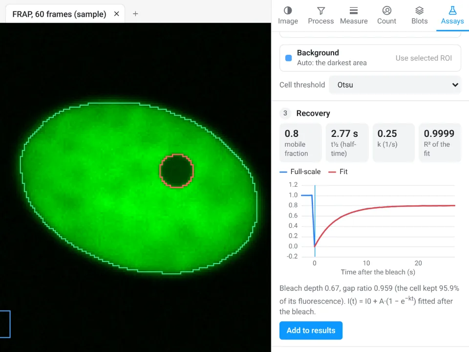
On the same movie LabCanvas gives mobile fraction 0.8 and t½ 2.77 s (R² 0.9999); ImageJ above gave 0.80 and 2.78 s.
Why switch for FRAP:
- A guided assay instead of a macro: bleach frame, regions, double normalisation and the fit in one panel, with the regions drawn on the image.
- Results straight to Graphs for comparing cells and conditions, with a methods sentence to copy.
- Nothing to install, and every measurement is checked in more than 4,000 automated tests.
Fiji stays better for models beyond a single exponential (reaction–diffusion fits, two populations) through scripts, and for reading .czi, .nd2 or .lif directly; LabCanvas needs those as OME-TIFF.
Open Image Analysis: free with a LabCanvas account (downloading files is part of LabCanvas Pro). ImageJ and Fiji are independent open-source projects; LabCanvas is not affiliated with them.
References
- Phair RD, Gorski SA, Misteli T (2004). Measurement of dynamic protein binding to chromatin in vivo, using photobleaching microscopy. Methods in Enzymology 375, 393–414. doi:10.1016/s0076-6879(03)75025-375025-3)
- Rapsomaniki MA, Kotsantis P, Symeonidou IE, Giakoumakis NN, Taraviras S, Lygerou Z (2012). easyFRAP: an interactive, easy-to-use tool for qualitative and quantitative analysis of FRAP data. Bioinformatics 28, 1800–1801. doi:10.1093/bioinformatics/bts241
- Schneider CA, Rasband WS, Eliceiri KW (2012). NIH Image to ImageJ: 25 years of image analysis. Nature Methods 9, 671–675. doi:10.1038/nmeth.2089
Frequently asked questions
How do I calculate the mobile fraction in FRAP?
How do I get the FRAP half-time?
Fit the recovery after the bleach with a single exponential,
What is double normalisation in FRAP?
It corrects the bleach-spot intensity for the background and for the fluorescence lost while imaging and in the bleach itself:
Why do I need a reference ROI in FRAP?
Imaging itself bleaches the sample a little in every frame, and the bleach removes part of the cell's fluorescence. Without a reference, the recovery curve peaks and then falls. On our example, leaving the reference out gives a mobile fraction of 0.60 and a half-time of 1.73 s instead of 0.80 and 2.78 s.
Is there a FRAP plugin for ImageJ?
Plain ImageJ needs no plugin: the ROI Manager, Multi Measure and Analyze › Tools › Curve Fitting cover it, with a few lines of macro for the normalisation. Fiji update sites and standalone tools such as easyFRAP add batch normalisation and fitting.
Is there an easier way without installing ImageJ?
LabCanvas Image Analysis has a guided FRAP recovery assay in the browser: it finds the bleach frame and the three regions, double normalises, fits the recovery and reports the mobile fraction and t½. It is free with a LabCanvas account.
Try it in LabCanvas
Every app is free to start in your browser. Create an account and begin.
Start Image Analysis free in your browserKeep reading
ImageJ vs LabCanvas Image Analysis: an honest comparison
ImageJ/Fiji or LabCanvas Image Analysis? Six everyday jobs done in both, six newer ones (macros, vendor files, 3D, StarDist, big images) and which to use.
How to use ImageJ: a beginner's tutorial for the 10 everyday jobs (2026)
How to use ImageJ and Fiji: get started, open an image, then 10 everyday jobs (scale, measure, threshold, count, background, blots) with exact menu paths.
How to set the scale and add a scale bar in ImageJ (with a calibration image to practise on)
Set the scale in ImageJ (Analyze › Set Scale) from a micrometer, scale bar or pixel size, add a scale bar, and practise on a free calibration image.