Nanoparticle size distribution from TEM images in ImageJ (step by step)
Nanoparticle size from TEM in ImageJ: scale, threshold, watershed, Analyze Particles with Feret, then the size histogram and mean ± SD, worked through.
Contents
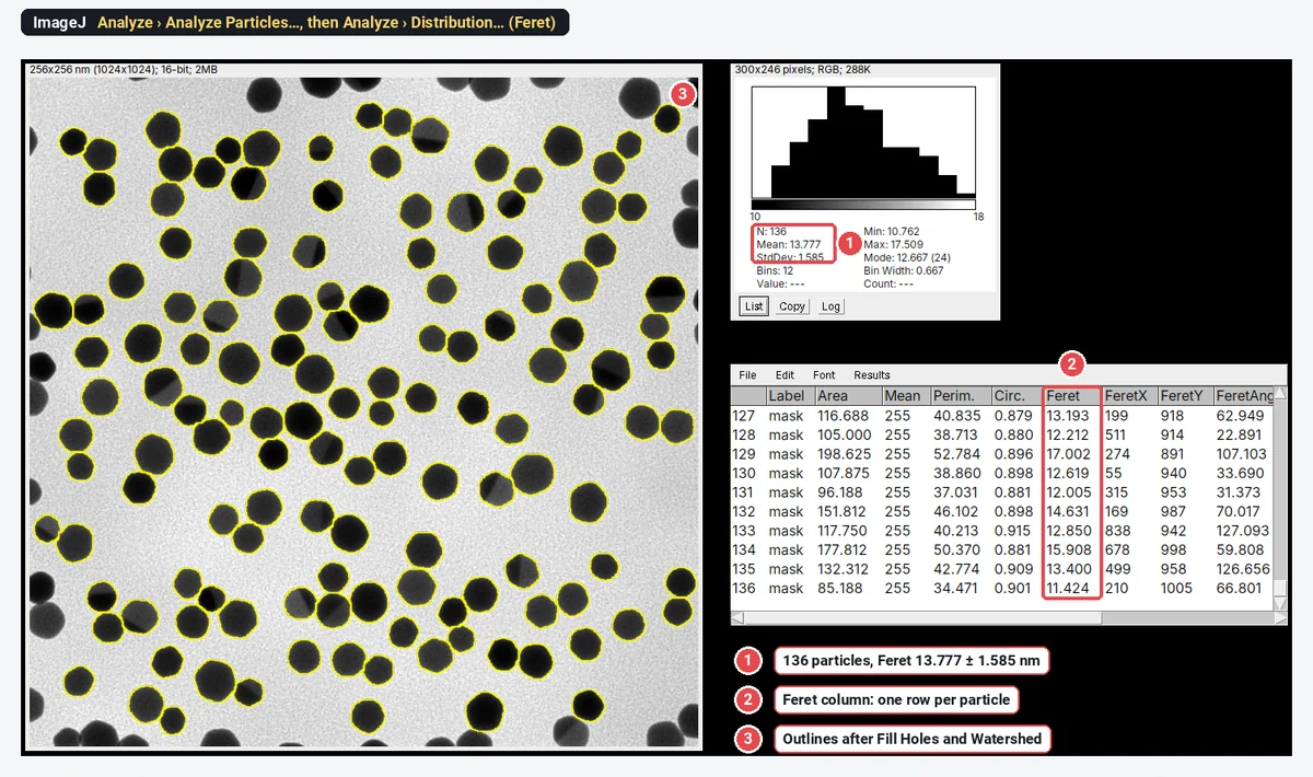
To get a nanoparticle size distribution from a TEM image in ImageJ, check the scale, threshold the dark particles, apply Fill Holes and Watershed to the mask, and run Analyze › Analyze Particles… with Feret's diameter ticked in Set Measurements and Exclude on edges on. Each Results row is one particle; Analyze › Distribution… on the Feret column gives the histogram, with n, mean and SD.
Worked example: on a sample TEM image of gold nanoparticles (synthetic, 1024 × 1024 pixels at 0.25 nm per pixel), ImageJ 1.54f measures 136 particles with a Feret diameter of 13.777 ± 1.585 nm (mean ± SD).
Before you start: image the particles so they can be measured
The analysis can only be as good as the image. Three things decide most of the result:
- Pixels per particle. Aim for at least 10 pixels across the smallest particle; 20 or more is better. Each outline is uncertain by about a pixel, so a 14 nm particle at 0.25 nm per pixel (55 pixels across) is measured to about 2%, while at 1.4 nm per pixel (10 pixels) the error is closer to 10%. The microscope pixel size calculator helps check what your magnification gives.
- Contrast and focus. Particles should be clearly darker than the support film, with sharp edges. A defocused edge spreads over several pixels and the threshold decides where it sits.
- Dispersion. Particles that overlap cannot be separated by any software. Dilute the sample or choose grid areas with separate particles, and take images in several places on the grid.
Pyrz and Buttrey (2008) work through these choices (bright or dark field, magnification, manual or automated analysis, and where the particle boundary lies) and how each one shifts the measured distribution.
In ImageJ (or Fiji), step by step
1. Open the image and check the scale
Open the original TIFF from the microscope, not a JPEG export or a screenshot. Then check Image › Properties…: if the pixel width is filled in with a unit (here 0.25 nm), the scale came with the file.
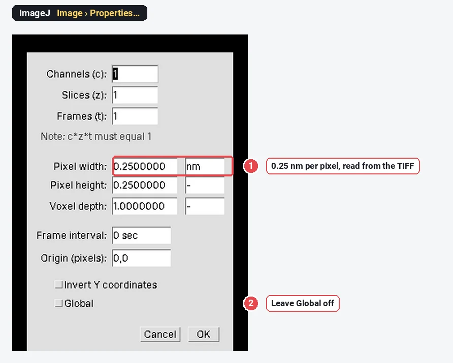
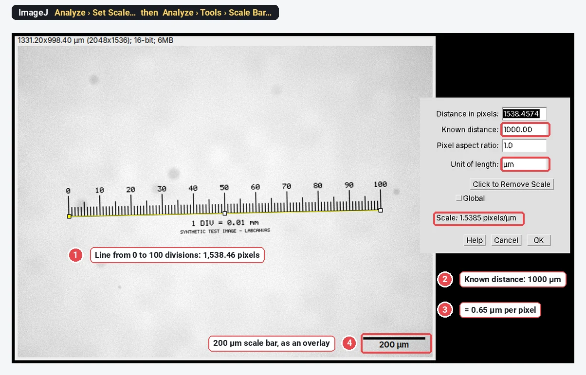
If the pixel width is 1 and the unit "pixel", ImageJ did not read the scale (some vendor formats keep it in their own header). Set it from the scale bar: draw a straight line along the bar, then Analyze › Set Scale…, type the bar length as the Known distance and nm as the unit. How to set the scale in ImageJ shows it step by step. Crop off any data bar with Image › Crop, so its text is not counted.
2. Threshold the particles
Open Image › Adjust › Threshold…. Gold particles in bright-field TEM are darker than the film, so untick Dark background, choose a method (Otsu is a good first try on a two-peaked histogram) and check that the red covers each particle to its edge and nothing else.
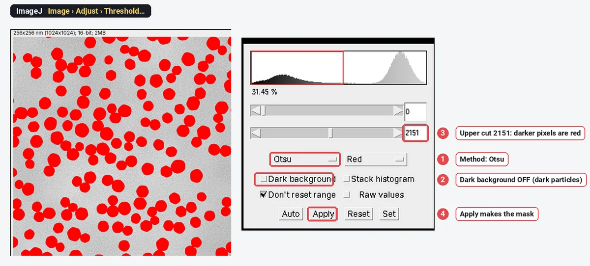
Zoom to 200% and look at a few edges. If the red stops short of the dark rim, the particles will be measured too small; if it spills into the halo, too large. With 16-bit images, the threshold window works on the raw values; there is no need to convert to 8-bit first.
3. Make a clean mask and split touching particles
- Click Apply (or Process › Binary › Convert to Mask).
- Process › Binary › Fill Holes: some particles have bright twin planes or noise inside; filling keeps them whole.
- Process › Binary › Watershed: cuts touching round particles apart at their necks.
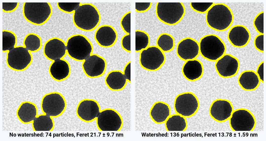
The watershed matters more than any other step on this image: without it, ImageJ counts 74 objects with a mean "diameter" of 21.7 ± 9.7 nm, because every touching pair is measured as one long particle. With it, 136 particles at 13.78 ± 1.59 nm. Check the cuts on the image: watershed separates round particles well, but it also cuts rods and irregular particles into pieces. More in watershed for touching particles.
4. Measure every particle
- Analyze › Set Measurements…: tick Area, Shape descriptors and Feret's diameter.
- Analyze › Analyze Particles…: Size 20-Infinity (in nm², since the image is calibrated), Circularity 0.00-1.00, Show Overlay or Outlines, and tick Display results, Clear results, Summarize and Exclude on edges.
- The Summary gives Count 136, Average Size 133.855 nm² and the mean Feret, 13.777 nm. The Results table has one row per particle.
Exclude on edges matters for size: particles cut by the frame are measured small. On this image it takes the count from 164 to 136. Every option of the dialog is in Analyze Particles in ImageJ, explained.
5. Draw the histogram and get mean ± SD
Choose Analyze › Distribution…, pick Feret as the parameter, and either tick Automatic binning or give the number of bins and the range (here 12 bins from 10 to 18 nm, so each bin is 0.667 nm wide).
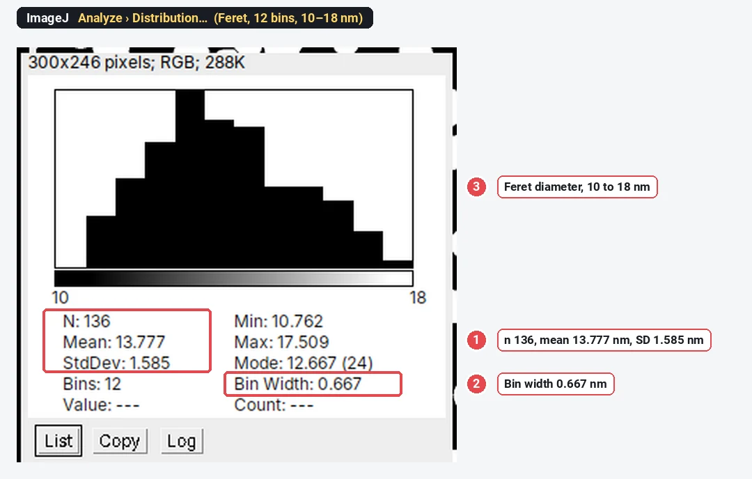
The window gives N, Mean, StdDev, Min, Max and the Mode. List writes the bin counts as a table, which you can copy into a plotting program for the figure. For the median and percentiles, sort the Feret column (Results › Sort) and read them off, or copy the column to a spreadsheet.
The result for the sample
| Statistic (n = 136) | Value |
|---|---|
| Mean Feret ± SD | 13.78 ± 1.59 nm |
| Coefficient of variation (SD/mean) | 11.5% |
| Standard error of the mean ( | 0.14 nm |
| D10, D50 (median), D90 of the Feret diameters | about 11.8, 13.6 and 16.1 nm |
| Range | 10.76 to 17.51 nm |
| Mean equivalent diameter, | 12.97 ± 1.52 nm |
| Mean MinFeret | 12.71 ± 1.49 nm |
Two numbers people mix up: the SD (1.59 nm) is the spread of the particles, the property of the sample; the standard error (0.14 nm) is the uncertainty of the mean, and it shrinks as you count more. Report the SD for the size distribution.
Feret diameter or equivalent diameter?
| Diameter | Definition | On the sample | Use it when |
|---|---|---|---|
| Feret | Longest calliper distance across the particle | 13.78 ± 1.59 nm | Faceted or slightly elongated particles; comparing with a ruler-tool measurement |
| Equivalent circle diameter | 12.97 ± 1.52 nm | Comparing with DLS, SAXS or other techniques that report a sphere-equivalent size | |
| MinFeret | Narrowest calliper width | 12.71 ± 1.49 nm | The short axis of rods, plates seen edge-on |
The three differ by 1 nm on the same particles, about 8%. None is wrong; the mistake is not saying which one you report. For near-spherical particles the equivalent diameter is the one most comparable with other techniques. Any TEM size, whichever definition, is the metal core: it will be smaller than a DLS hydrodynamic diameter, which includes the ligand shell and the solvent around it. The shape columns are explained in Feret diameter, circularity and solidity.
How many particles should you count?
The precision of the mean depends on the spread and the count. For a 95% margin
With the sample's SD of 1.585 nm:
| Margin on the mean | Particles needed |
|---|---|
| ± 0.5 nm | about 40 |
| ± 0.2 nm | about 240 |
| ± 0.1 nm | about 970 |
The 136 particles here give the mean to about ±0.27 nm. That covers the random error only. The systematic errors (threshold position, scale calibration, which particles landed in the images) do not shrink with n, so take images from several places on the grid, and from more than one grid when you compare batches. A few hundred particles from five or more images is a common, defensible target; for the shape of the distribution (tails, a second population), count more.
Touching and overlapping particles
- Touching, round particles: watershed separates them, as above. Check the cuts.
- Overlapping particles (one partly on top of another): the overlap is darker, but the outline of the lower particle is gone. Watershed cuts them somewhere plausible, not at the true boundary. Exclude them (a solidity filter below about 0.9 catches most merged pairs), or measure a few by hand with the line tool to check.
- Aggregates: exclude them from the size distribution and report the fraction of aggregated particles separately if it matters.
- Rods, plates and irregular particles: leave watershed off. Count them separately with Feret (length) and MinFeret (width).
Zhang and Wang (2023) published a step-by-step protocol for this job: the size distribution of silica nanoparticles measured from a TEM image with ImageJ 1.53t. It is a useful citation for the method.
Pitfalls
- JPEG or screenshot instead of the TIFF. Compression blurs edges and the scale can be lost. Use the original file.
- A scale bar read by eye. On a 1024-pixel image, a scale bar line a few pixels off is a 1–2% error on every size. Prefer the pixel size stored in the file.
- The threshold sets the size. Every particle grows or shrinks by about a pixel all round as the cut moves: here that is 0.5 nm on every diameter. Use one method for a series and say which.
- Uneven background. A darker corner can pull the threshold. Process › Subtract Background… (light background ticked, radius larger than the largest particle) or a manual threshold per image helps.
- Edge particles counted. Without Exclude on edges, cut particles pull the mean down (here the mean area falls from 133.9 to 124.9 nm²).
- Dust and noise counted. Set a minimum size from the image; on this sample anything from 5 to 50 nm² gives the same 136 particles.
Reporting it
A methods sentence to adapt:
Particle sizes were measured from bright-field TEM images (0.25 nm per pixel) in ImageJ 1.54f (Schneider et al., 2012), following Zhang and Wang (2023). Particles were segmented with the Otsu threshold, holes were filled and touching particles separated with the watershed algorithm; particles smaller than 20 nm² or touching the image edge were excluded. The Feret diameter of each particle was measured; we report mean ± SD (n = 136 particles from one image).
Show the histogram with the bin width stated, the mean ± SD and n (particles and images) in the caption, and a representative TEM image with a scale bar (Analyze › Tools › Scale Bar…; Image › Overlay › Flatten burns the outlines in).
Where ImageJ and Fiji do more
For hundreds of images, an ImageJ macro runs these steps unattended: record one image with Plugins › Macros › Record…, then run it on a folder with Process › Batch › Macro…. For crowded or overlapping particles, Fiji plugins such as StarDist (round objects) or Trainable Weka Segmentation separate what a threshold cannot; for 3D tomograms, Fiji has 3D tools.
An easier way: particle sizes in LabCanvas
LabCanvas Image Analysis does the threshold, fill, watershed and count in one panel, in the browser, on the raw 16-bit values, with nothing to install.
- Open the TIFF; the 0.25 nm pixel size is read from it.
- Tick Area and Feret's diameter in Measure › Set measurements.
- In Count › Count particles: threshold Otsu, objects Dark, tick Fill holes, Separate touching objects (watershed) and Exclude particles on the edges, smallest particle 20 nm². The threshold preview updates live.
- Click Count, then Send to Graphs with the Feret column and All rows for the histogram and descriptive statistics (mean, SD, median, n).
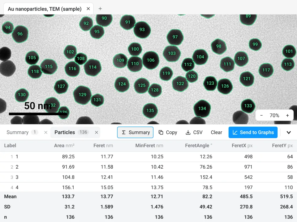
On the same file: 136 particles, Feret 13.77 ± 1.589 nm, against 136 and 13.777 ± 1.585 nm in ImageJ. The two watershed implementations split a few touching pairs a pixel differently, and the means agree to 0.01 nm.
Why it is a good choice for TEM sizing:
- One panel instead of five commands: threshold, Fill holes, watershed, size limit and edge exclusion together, with a live preview.
- An image check first: it warns about clipping, JPEG compression and uneven illumination before you measure.
- The histogram without a spreadsheet: Send to Graphs makes the size distribution; for equivalent diameters, send Area and transform it with Y = 2*sqrt(Y/pi).
- A methods sentence: the Methods button above the table writes the measurement part, and Add image to canvas places the image with its outlines and scale bar in a figure.
- Checked: every measurement is validated against independent software in more than 4,000 automated tests.
It has Count › Batch for many images but no macro language, and no StarDist. Image Analysis is free with a LabCanvas account; downloading CSV files is part of LabCanvas Pro. Open Image Analysis. ImageJ and Fiji are independent open-source projects; LabCanvas is not affiliated with them.
References
- Zhang S, Wang C (2023). Precise analysis of nanoparticle size distribution in TEM image. Methods and Protocols 6(4): 63. doi:10.3390/mps6040063
- Pyrz WD, Buttrey DJ (2008). Particle size determination using TEM: a discussion of image acquisition and analysis for the novice microscopist. Langmuir 24(20): 11350–11360. doi:10.1021/la801367j
- Schneider CA, Rasband WS, Eliceiri KW (2012). NIH Image to ImageJ: 25 years of image analysis. Nature Methods 9(7): 671–675. doi:10.1038/nmeth.2089
Frequently asked questions
How do I measure nanoparticle size from a TEM image in ImageJ?
Check the scale (Image › Properties), threshold the particles (Image › Adjust › Threshold, Dark background off for dark particles), Apply, then Process › Binary › Fill Holes and Watershed. Tick Area and Feret's diameter in Analyze › Set Measurements and run Analyze › Analyze Particles with a small minimum size and Exclude on edges. Each row of the Results table is one particle; Analyze › Distribution… draws the histogram.
How many nanoparticles should I measure for a size distribution?
Enough that the mean is known to the precision you need:
Should I report Feret diameter or equivalent circle diameter?
Either, but say which. Feret is the largest calliper distance and suits faceted or slightly elongated particles; the equivalent diameter,
How do I separate touching nanoparticles in ImageJ?
Make a binary mask, fill holes and run Process › Binary › Watershed, which cuts touching round particles at their necks. On our sample it takes the count from 74 merged objects to 136 particles. It does not work on heavily overlapping particles or long rods; leave those out or measure them by hand.
How do I make a particle size histogram in ImageJ?
After Analyze Particles, choose Analyze › Distribution…, pick the Feret column, and either use automatic binning or set the number of bins and the range. The window shows the histogram with n, mean, SD, min, max and the mode. For a publication figure, copy the Results to a plotting program.
Is there an easier way to get a particle size distribution?
Yes: Count particles in LabCanvas Image Analysis does the threshold, fill, watershed and count in one panel in the browser, and sends the Feret column to a histogram; see the last section of this guide.
Try it in LabCanvas
Every app is free to start in your browser. Create an account and begin.
Start Image Analysis free in your browserKeep reading
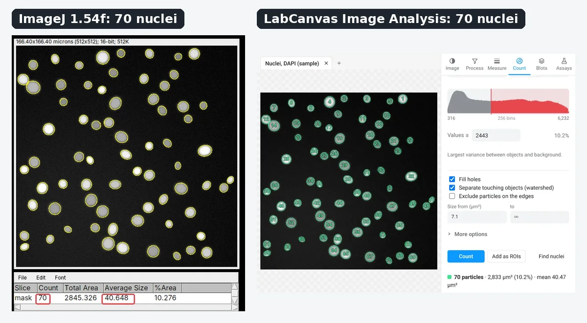
ImageJ vs LabCanvas Image Analysis: an honest comparison
ImageJ/Fiji or LabCanvas Image Analysis? Six everyday jobs done in both, six newer ones (macros, vendor files, 3D, StarDist, big images) and which to use.
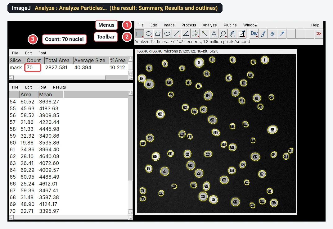
How to use ImageJ: a beginner's tutorial for the 10 everyday jobs (2026)
How to use ImageJ and Fiji: get started, open an image, then 10 everyday jobs (scale, measure, threshold, count, background, blots) with exact menu paths.
How to set the scale and add a scale bar in ImageJ (with a calibration image to practise on)
Set the scale in ImageJ (Analyze › Set Scale) from a micrometer, scale bar or pixel size, add a scale bar, and practise on a free calibration image.